Parametric Dirac Delta to Simplify the Solution of Linear and Nonlinear Problems with an Impulsive Forcing Function ()
1. Introduction
The purpose of this paper is to present a more rigorous derivation of the parametric Dirac delta than that which was presented in [1], and also to illustrate its application in partial differential equations and nonlinear problems.
According to distribution theory, the Dirac delta is the result of differentiating the Heaviside unit step. The particular parameterization presented in [1] permits this differentiation to be carried out by means of elementary calculus and the resulting pair of parametric equations are exact and closed.
The delta equations have the same function values as those specified in the definition; the area involved has a unit value; they comply with the fundamental property and yield the correct Laplace and Fourier transforms [1]. In the solution of differential equations, they are handled exclusively by calculus and algebra, both at an elementary level. The parameterized representation can be readily visualized geometrically. These two features should make these parametric equations particularly convenient as a useful research tool, and also, for the purpose of teaching the Dirac delta concept at an early stage in undergraduate school.
2. Basic Concepts
For the sake of simplicity and readability, in this paper, the Dirac delta will be derived and applied considering it to represent a time concentration, and not a space concentration, and that the point of concentration occurs at time equal to zero, i.e., in the form often referred to as the “Impulse Function”.
2.1. Various Unit Steps
There are three different definitions of the Heaviside unit step in common use [2-6]:
 (1)
(1)
see Figure 1.
2.2. The Cauchy Limiting Coefficient
Cauchy proposed a limiting coefficient and represented it by the following equation [7]:
 (2)
(2)
This coefficient he used to delimit the interval of validity of a function.
It is worth pointing out that both in the third definition of the Heaviside unit step, Equation (1), and in the Cauchy limiting coefficient, Equation (2), the value of the jump point is undefined; as a matter of fact, their graphical representation is identical, Figure 1. However, they differ in that the derivative of the Cauchy coefficient is zero, it is not the Dirac delta, this is easily confirmed by Mathematica, Maple and by the TI 92 calculator.
2.3. Unit Step with a Riser
Consider a variant of the Heaviside unit step which, unlike it, the jump point is filled with a vertical straight line. We will call this the unit step with a riser, HR, Figure 2.
3. Derivation of the Parametric Dirac Delta
Consider the approximation of the unit step with a near vertical riser, HRa, shown in Figure 3.
It is clear that:
 (3)
(3)
From Figure 3, the equation for HRa is easily established:
 (4)
(4)
Notice that, in this paper, λ is used as a switch, i.e., to switch on functions at the beginning of their interval of validity and to switch them off at the end of their interval of validity. In this manner, various different functions are linked together into a single composite function.
3.1. Parametric Representation
Figures 4 and 5 together are the parametric representa-

Figure 1. Graphical representation of both the third definition of the Heaviside unit step, Equation (1), and the Cauchy limiting coefficient, Equation (2). Note: Matlab was used for this plot because, unlike other software, it does not leave a trace at the jump point.

Figure 3. Approximate unit step with a riser.

Figure 4. Unit step with a near vertical riser HRa as a function of the parameter w.

Figure 5. Approximate time ta versus the parameter w.
tion of HRa, with the length of the curve w as the parameter.
From Figures 4 and 5 we obtain the equations:
 (5)
(5)
 (6)
(6)
These two functions would be continuous were it not for the fact that they are undetermined at the points
 and
and , however, since their left limit is the same as their right limit at those points, they will be treated as if they were continuous because this “··· is generally inconsequential in applications”, [6], see also [4,5,7]. This is true also for most of the functions contained in the equations in the rest of this paper. It is significant that this conversion of a discontinuous function into a “continuous” function by means of a parameterization has been used also to eliminate the Gibbs phenomenon [8].
From this point on, all the derivatives have been verified by using Mathematica.
Differentiating Equations (5) and (6):
 (7)
(7)
 (8)
(8)
Now:
 (9)
(9)
Carrying out the slash division in a piecewise fashion yields:
 (10)
(10)
or simply
 (11)
(11)
and
 (12)
(12)
which means:
 (13)
(13)
but this is the Dirac delta,
 (14)
(14)
But also,  may be expressed as:
taking the limit yields:
 (16)
(16)
in accordance with Equation (14):
 (17)
(17)
Taking the limit of  as
as  of Equation (6) yields:
|  (15) (15) |
 (18)
(18)
Thus the pair of Equations (17) and (18) is the parametric representation of the Dirac delta. However, an abbreviated version of these equations for the application referring to the impulse function will be established in Section 3.4.
3.2. Illuminating Plots
Some very illuminating plots result if we invert the order of the operations on parametric Equations (5) and (6), i.e., we first carry them to the limit as , Figures 6(c) and (d), and we differentiate them afterwards, Figures 6(e) and(f).
1st Step. Carrying them to the limit yields:
 (19)
(19)
 (20)
(20)
see Figures 6(c) and (d).
2nd Step. Differentiating Equations (19) and (20) yields:
 (21)
(21)
 (22)
(22)
see Figures 6(e) and (f).
Substituting Equations (21) and (22) into Equations (9) and (14) yields Equation (17), thus confirming it.
Figures 6(a)-(d), illustrate the process of converting the unit step function into a virtually continuous function. Figure 6(a) illustrates the usual unit step with a gap at the jump point. Figure 6(b)" target="_self">Figure 6(b)" target="_self"> Figure 6(b)" target="_self">Figure 6(b) shows the fundamental idea of a unit step with a riser, the parameter w is the length along this function. Figures 6(c) and (d) represent the parameterized unit step with a riser, these are the plots of the resulting virtually continuous functions. It is significant that the single point,  , of Figure 6(b)" target="_self">Figure 6(b) has been expanded into the finite interval,
  , in Figures 6(c)-(f).
3.3. Displaced Point Plots
If we now plot
 and
and 
versus t, and not versus w, the finite intervals, from 0 to 1, of Figures 6(e) and (f) become the single points  of Figures 7(a) and (b). As can be seen in Figure 7(c), even though, the scale of the ordinate is very compressed (up to 10 × 1030), no displaced point appears since it is

Figure 6. (a) Plot of either the Heaviside unit step, H(t − 0), third version, Equation (1), or Cauchy’s limiting coefficient, λ(t − 0), Equation (2). (b) Parametric plot of the unit step with a riser, Equation (19) versus Equation (20). (c) Plot of Equation (20). (d) Plot of Equation (19). (e) Plot of Equation (22). (f) Plot of Equation (21). Note: Matlab was used for these plots because it makes a clear distinction between the step with a riser and the step without a riser and so does the TI 92 graphics calculator. A plot of the riserless step, Figure 6(a), in another software or another graphics calculator may result in a trace at the jump point making it indistinguishable from the step with a riser.

Figure 7. (a) Plot of Equation (21) versus Equation (20). (b) Plot of Equation (22) versus Equation (20). The plots (a) and (b) may be called displaced point plots. The circles help to locate the gaps which are very narrow and the points which are very faint. (c) Plot of Equation (17) versus Equation (18).
located at infinity.
3.4. Plot of a True Single Point
It is interesting to compare Figures 7(a) and 8, both are plots of Equation (21) versus Equation (20), but the plotting increment of Figure 8 is much greater than that of Figure 7(a), and consequently the gap of Figure 8 is also much greater than that of Figure 7(a). Notice however,

Figure 8. Direct plot of Equation (21) versus Equation (20), with a very large plotting increment. Notice that the gap is much larger than in plot 7(a), however the displaced point remains the same size and just as faint since it is truly a single point.
that the size of the displaced point remains the same, since it really refers to a single point.
Considering that there is no negative time, the plots of Figure 6 are conveniently substituted by those of Figure 9.
From Figure 9 we obtain the following abbreviated equations:
 (23)
(23)
 (24)
(24)
 (25)
(25)
 (26)
(26)
 (27)
(27)
 (28)
(28)
Thus the remarkably simple pair of parametric Equation (28) represent what is often called the “impulse function”. These are the equations to be used in the solution of problems.
4. Examples
4.1. Example 1
Consider a one dimensional rod subject to an impulsive heat source with initial temperature of 0˚C along its full

Figure 9. These plots lead to the representation of the impulse function, Equations (23) to (28), and they are obtained by simply cutting off the negative time. The pertinent equations are obtained from these plots. (a) Parametric plot of HR(w − 0), Equation (24) vs. t, Equation (23). (b) Plot of Equation (23). (c) Plot of Equation (24). (d) Plot of Equation (27). (e) Plot of Equation (26).
length and with the ends kept at 0˚C throughout the whole process. The governing equation is:
 (30)
(30)
(here q has units of energy/volume)
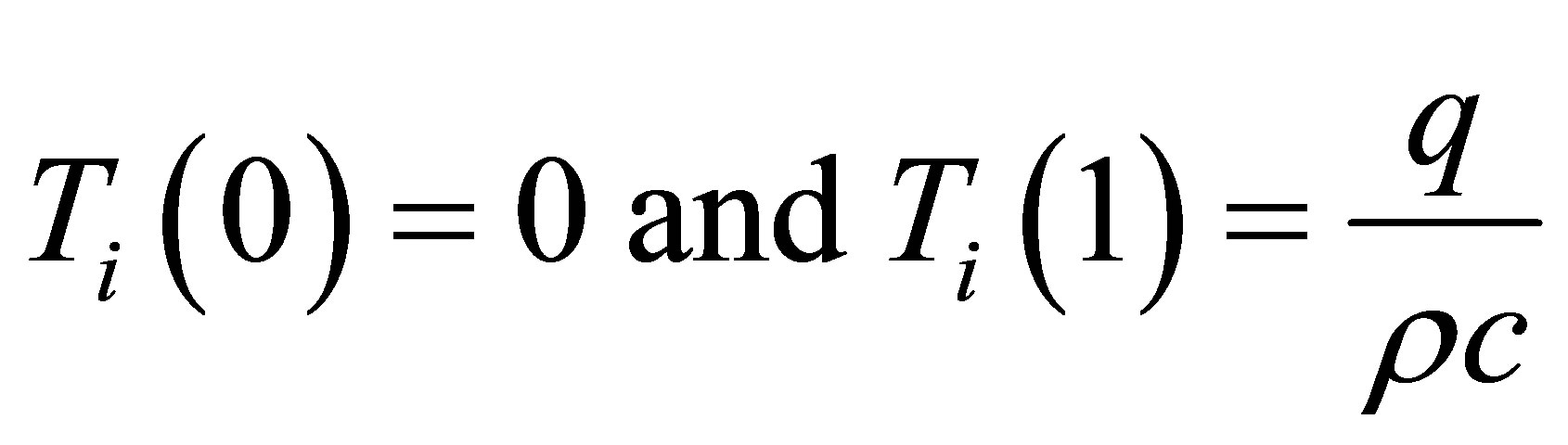
Subject to the boundary conditions:
 (31)
(31)
and to the initial condition:
 . (32)
Nomenclature:
c = coefficient of heat transfer;
k = conductivity;
 ;
;
Q = heat energy;
m = mass;
T = temperature;
t = time;
V = volume;
x = position along the rod;
 mass density.
Following the method of separation of variables [9]:
 . (33)
Substituting Equations (25) and (33) into Equation (30) yields:
 . (34)
Introducing the parameter w into Equation (34):
 (35)
(35)
multiplying Equation (35) by :
:
 (36)
(36)
Substituting Equations (26) and (27) into Equation (36), yields what we will call the control equation:
 (37)
(37)
4.1.1. Impulse Instant
During the impulse instant, designated as interval i,  ,
,  , Equation (23), accordingly Equation (37) becomes
 , (38)
or according to Equation (33):
 (39)
(39)
Comparing Equation (39) with the original differential Equation (30) it stands out that, during the impulse instant, the term referring to conduction is absent. This is as it should be, since there is no time for conduction to take place, in perfect agreement with physical reality. Also the Dirac delta, as such, is absent and the forcing function is simply a constant.
Dividing Equation (38) by :
:
 (40)
(40)
where  is a separation constant, then
 (41)
(41)
integrating:
 (42)
(42)
Substituting Equations (42) into Equation (33):
 (43)
(43)
At the “beginning” of the impulse instant, w = 0, and according to the initial condition, Equation (33), . Substituting this into Equation (43) requires that:
 (44)
(44)
and thus Equation (43) reduces to:
 .(45)
.(45)
Equation (45) governs during the impulse instant, thus:
 (46)
(46)
the change of temperature during the impulse instant is
 (47)
(47)
but  and
and , substituting these values in Equation (47) yields:
 , (48)
since m remains constant, we have the principle
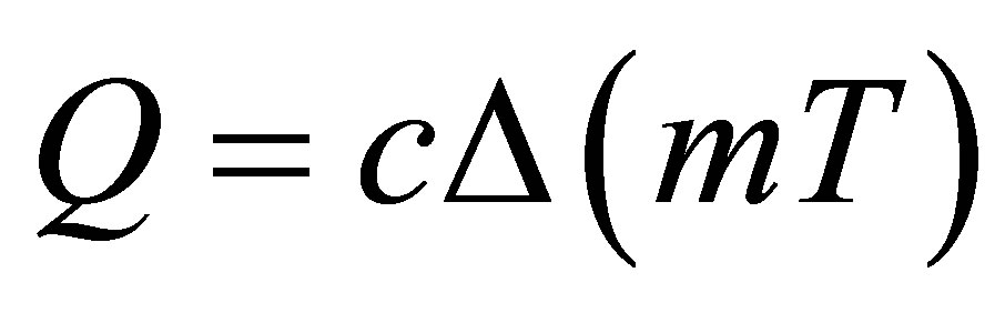 (49)
(49)
or in words: “The heat impulse is equal to the change in sensible heat”.
This is somewhat similar to the mechanical impulse and change in momentum principle.
4.1.2. Post Impulse Time
At post impulse time, designated as interval p, w ≥ 1,  , Equation (23), and thus Equation (37) becomes:
 . (50)
Physical considerations require that:
 (51)
(51)
To make things clear, it is convenient to emphasize that:
 (52)
(52)
But in this interval,  , substituting this and making use of Equation (33), Equation (50) is equivalent to the following homogeneous equation:
 . (53)
and in view of the second of Equations(46) and Equation (51), the initial temperature of post-impulse time is:
 (54)
(54)
and, of course, the boundary conditions are the same as the original ones, Equation (31), thus:
 (55)
(55)
The problem made up of Equations (53)-(55) has the well known conventional solution, see for instance [9]:
 (56)
(56)
see plot, Figure 11.
4.1.3. The Complete Solution
Using Equations (45) and (56) the complete parametric solution is obtained thus:
 (57)
(57)
Notice that the first term of Equation (57) is the impulse instant solution and the second term is the post impulse solution.
Notice that since t is a function of w, both Equations (57) are functions only of the parameter, w. See Figure 10.
It is interesting to compare the plot of the parametric solution, Equation (57), Figure 10(a), with the plot of the conventional solution Equation (56), Figure 11. The parametric solution clearly shows the initial condition to be zero, i.e.,  , strictly in accordance with the specified condition, Equation (32), and, furthermore it shows the initial, instantaneous process of the change of temperature, i.e.:
 , while the plot of the conventional solution shows the initial temperature to be
 , which is not in agreement with the specified condition, Equation (32). Also in Figure 11 the pseudo initial condition is plagued by the spurious oscillations due to the Gibbs phenomenon.
4.2. Example 2
Consider a mass-spring non-linear system subjected to an initial impulse where the spring force is given by:
 (58)
(58)
as in the Duffing equation.


Figure 10. Plots of the parametric solution, Equations (57). (a) “Front view” plot. Notice that the instantaneous change of the value of the temperature from its initial value, 0, to 1 (in non-dimensional terms) is clearly shown by the front “wall” which is not present in the plot of the conventional solution, Figure 11. (b) “Rear view” plot.
 , (59)
with initial conditions:
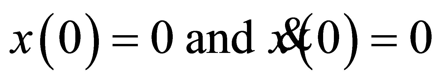 (60)
(60)
I is the magnitude of the impulse.
Converting the second order Equation (59) into two first order equations by means of the state variables:
 (61)
(61)
Introducing the parameter w into Equation (61):

Figure 11. Plot of the conventional solution, Equation (56). The value of the initial temperature was given as zero, but in this plot it is shown as one (dimensionless) and the instantaneous change of temperature process that takes place during the impulse instant (the “wall” of Figure 10(a)) is not shown. The oscillations in the value of the pseudo initial temperature along the full length of the rod are spurious, they are due to the Gibbs phenomenon. Compare this with the plot of the parametric solution, Figure 10.
 (62)
(62)
multiplying by :
:
 (63)
(63)
substituting Equations (26) and (27) into Equation (63) yields the control equations:
 (64)
(64)
4.2.1. Impulse Instant
During the impulse instant: , Equation (23), and thus Equations(64) become:
 (65)
(65)
(The subscript i refers to the impulse instant).
Notice that the parameterization resulted in the simplification of the forcing function which is now simply the constant I, i.e., the Dirac delta, as such, is absent from the previous equations. Also absent is the term referring to the spring force, thus representing faithfully the physical reality, i.e., during the impulse instant, there is no time for the displacement of the mass, and thus the spring does not participate in this process.
Integrating Equations (65):
 (66)
(66)
from the initial conditions the integration constants are evaluated, thus:


and, therefore, the governing equations for the impulse instant are:
 (67)
(67)
and so at the “end” of the impulse instant, i.e., at 
 , Equation (23):
 (68)
(68)
The 2nd of Equations (67) states that there is no motion during the impulse instant.
Now
 (69)
(69)
 (70)
(70)
This is the principle of impulse and momentum and it was applied automatically by virtue of the parameterization.
4.2.2. Post Impulse Time
At post-impulse time (designated as interval P): 
 Equation (23), and thus Equation (64) become:
 (71)
(71)
In this interval:  and thus
 . Consequently, Equations (71) become:
 (72)
(72)
It is convenient to reduce the pair of Equations (72) into the single equation:
 (73)
(73)
Resorting to Equations (68) we establish the initial conditions of post-impulse time:
 , (74)
the phase-plane solution of Equation (73) is
 (75)
(75)
At this point it is convenient to use dimensionless variables:
 . (76)
In terms of these variables Equation (75) becomes
 (77)
(77)
Thus the complete phase-plane solution may be expressed as:
 (78)
(78)
In the first of Equations (78) the first term refers to the impulse instant and the second term refers to the post impulse time.
See Figure 12.
Equation (77) leads to:
 (79)
(79)
the solution of Equation (79) is the hypergeometric function
 (80)
(80)
see Figure 13(a).
From Equation (77):

Figure 12. Plot of the phase-plane solution.

Figure 13. (a) Time vs. displacement plot, (b) Time vs. velocity plot.
 (81)
(81)
Substituting Equation (81) into Equation (80) yields:
 (82)
(82)
see Figure 13(b).
Equations (80) and (82) may not be considered a convenient analytical solution; however their plots, Figure 13, make up a useful graphical solution.
5. Conclusions
The parametric representation of the Dirac delta as proposed in [1] has been reviewed with the purpose of clarifying the concept.
The parametric Dirac delta, contained in the forcing function of a differential equation referring to an impulsive process, has an operator action that splits this equation into two: the first referring to the impulse instant and the second referring to post-impulse time. In the impulse instant, the operator action converts the delta forcing function into a constant; and furthermore, it cancels the terms referring to the phenomena that cannot take place instantaneously.
Also, the operator action makes the post-impulse equation homogeneous. All of this makes the process of obtaining the solution considerably easier. As it has been mentioned before, in the case of Example 1 referring to the metal rod heated impulsively, the term associated with heat conduction disappears from the impulse instant equation. This is reconciled with the physical reality, i.e., there is no time for this process to take place.
In the case of the second order mass-nonlinear spring problem of Example 2, the term representing the spring force disappears from the impulse instant equation. This illustrates the faithfulness of the mathematical model, since in the impulse instant there is no time for the displacement of the mass to take place.
In Examples 1 and 2, the parametric representation permits the separation of variables even though the original differential equations are non-homogeneous.
In the parametric solution, the real initial conditions are used and the processes that take place during the impulse instant are fully represented as such. In contrast to this, in the solution of problems involving impulsive processes in some textbooks, the forcing function is sometimes replaced by equivalent initial conditions [10].
During the impulse instant: time, t, does not flow, but pseudo-time (parametric time), w, does flow and this is what makes possible the establishment of the equations that represent the processes that take place instantaneously.
In the parametric solution, the impulse instant becomes a finite interval in terms of the parameter. Thus there is no need to deal with infinitesimals.
This parametric representation may be taught at an earlier stage because the principle on which it is based is easily visualized geometrically and because it is only necessary to have a knowledge of elementary calculus to understand it and use it.
By virtue of the parametric representation of the Dirac delta, the principle of impulse and momentum was applied automatically in Example 2, also in Example 1 a similar result was obtained: the heat impulse is equal to the change in sensible heat. This suggests that the parametric representation of the Dirac delta may turn out to be a valuable research tool.