Forward-Backward Synergistic Acceleration Pursuit Algorithm Based on Compressed Sensing

Bowen Zheng, Guiling Sun^*, Tianyu Geng, Weijian Zhao

College of Electronic Information and Optical Engineering, Nankai University, Tianjin, China.

DOI: 10.4236/jcc.2017.510004                

Abstract

We propose the Forward-Backward Synergistic Acceleration Pursuit (FBSAP) algorithm in this paper. The FBSAP algorithm inherits the advantages of the Forward-Backward Pursuit (FBP) algorithm, which has high success rate of reconstruction and does not necessitate the sparsity level as a priori condition. Moreover, it solves the problem of FBP that the atom can be selected only by the fixed step size. By mining the correlation between candidate atoms and residuals, we innovatively propose the forward acceleration strategy to adjust the forward step size adaptively and reduce the computation. Meanwhile, we accelerate the algorithm further in backward step by fusing the strategy proposed in Acceleration Forward-Backward Pursuit (AFBP) algorithm. The experimental simulation results demonstrate that FBSAP can greatly reduce the running time of the algorithm while guaranteeing the success rate in contrast to FBP and AFBP.

Keywords

Compressed Sensing, Reconstruction Algorithm, Sparse Signal, FBP

1. Introduction

The theory of Compressed Sensing (CS) [1] [2] [3] proposed by Candes and Donoho in 2006, breaks the limitation that the traditional sampling must satisfy the Nyquist frequency and makes it possible to reconstruct low sampling rate signal. Therefore, CS is widely used in wireless sensor networks [4] [5] , magnetic resonance imaging [6] and video compression [7] etc.

The major research direction of CS includes signal sparse transformation, design of measurement matrix and signal reconstruction algorithm. The reconstruction algorithms are divided into three categories: greedy algorithms, relaxation algorithms and hybrid algorithms. Greedy algorithms are built upon a series of locally optimal single-term updates, including Matching Pursuit (MP) [8] and Orthogonal Matching Pursuit (OMP) [9] etc. Relaxation algorithms are based on convex optimization techniques, which can smooth the $l_0$ norm and replace it with a continuous function that can be handled using classic optimization, including Basis Pursuit (BP) [10] and Iterative Reweighted Least-Squares (IRLS) [11] etc. Hybrid algorithms include Subspace-Pursuit (SP) [12] , Compressive Sampling Matching Pursuit (CoSaMP) [13] and Iterative Hard Thresholding (IHT) [14] etc.

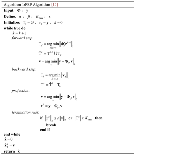
FBP is a novel two-stage greedy approach proposed by N. B. Karahanoglu and H. N. Erdogan in reference [15] . It enlarges the estimated support set by $\alpha$ atoms in forward step and eliminates $\beta$ atoms from the estimated support set in backward step. The disadvantage of the FBP is that it can only enlarge and reduce the estimated support set with a fixed step size. In view of this, Paper [16] proposed Acceleration Forward-Backward Pursuit (AFBP) algorithm, selected the high quality atoms again in backward step. Based on this, we propose the Forward-Backward Synergistic Acceleration Pursuit (FBSAP) algorithm in this paper, which can reduce the atoms selected in the forward step adaptively according to the quality of atoms. Thus the algorithm is further accelerated when we restructure sparse signals, especially the signals which have large amount of data. This greatly improves the practicability of reconstruction algorithms.

The remainder of the paper is organized as follows. Section 2 briefs the theory of CS and the FBP algorithm. Section 3 introduces the acceleration strategy we used and the specific process of FBSAP. Section 4 presents the simulation results. Finally, conclusion is present in Section 5.

2. Compressed Sensing Theory and Recovery Algorithm

2.1. The Theory of Compressed Sensing

Compressed Sensing aims at restructuring the signal by excavating its sparse feature when the information is sampled in very low sampling rate. The sampling process is represented by

$y=\Phi x$ (1)

where $x$ is a K-sparse one-dimensional signal of length N, K is the number of nonzero elements in $x$ . $\Phi$ is a $M\times N$ two-dimensional observation matrix with $K<M<N$ . $y$ is a one-dimensional measurement vector of length M. The purpose of CS is to obtain the signal $x$ by using the measurement vector $y$ and the observation matrix $\Phi$ .

2.2. The Forward-Backward Pursuit Algorithm

Without the sparsity K to be known a priori, FBP can reconstruct the sparse signal exactly by selecting atoms with fixed forward and backward step size in contrast to other reconstruction algorithms. The pseudo code of the FBP is given in Algorithm 1. It expands the estimated support set by selecting $\alpha$ atoms with highest correlation in the forward step and reduces the size of the estimated support set by eliminating $\beta$ atoms with smallest contributions to the projection.

3. Forward-Backward Synergistic Acceleration Pursuit Algorithm

3.1. The Acceleration Strategy

The FBP algorithm can be accelerated by two ways: reducing $\alpha$ and enlarging $\alpha -\beta$ . The strategy mentioned in [16] has the effect of enlarging the $\alpha -\beta$ , but it doesn’t change the number of atoms selected in the forward step.

It is not every atom selected in the forward step correct. The wrong atoms are more if the signal is very sparse or after many iterations. A fixed number of atoms are selected in every forward step that increases the computation. We observed the correlation levels of the observation matrix and residuals at first. The results are shown in Figure 1. We found that the correlation levels

(a) (b)

Figure 1. The correlation levels of the observation matrix and residuals. (a) The correlation level in first iteration; (b) The correlation level after some iterations.

present ladder-form. Some atoms have the same correlation level such as atoms 2-5, and there is a big ladder between them and the other atoms. The ladder is especially obvious after some iterations. The correlation level of atom 1 is significantly higher than the others. With the above analysis, it is completely unnecessary selecting $\alpha$ atoms in every iteration. Only need to find the last obvious ladder and choose the atoms before it. We can reduce $\alpha$ by this way and accelerate the algorithm.

We adopt the backward acceleration strategy proposed by [16] in this paper. The main idea of this strategy is giving the atoms corresponding weights according to the correlation levels between atoms and residuals, and then resetting the atom into support set in backward step if its cumulative weight is greater than a threshold, so that we can select multiple atoms in each iteration.

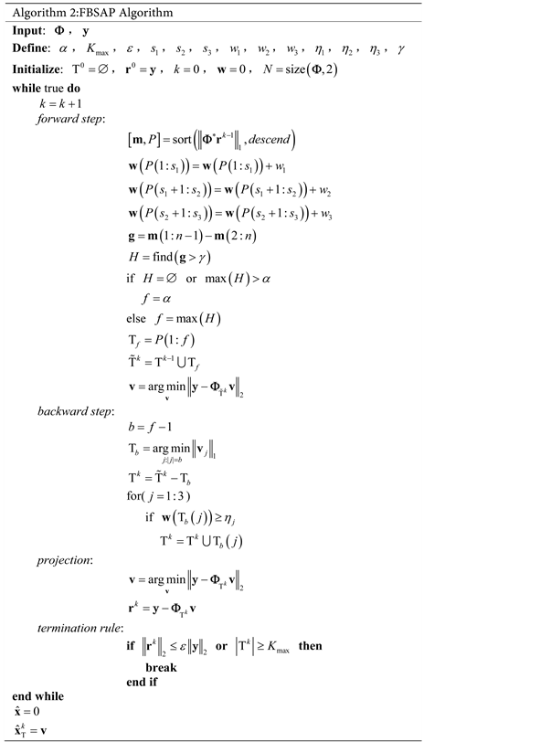
3.2. Forward-Backward Synergistic Acceleration Pursuit Algorithm

The details of FBSAP are shown in Algorithm 2. First, Calculate the correlation levels between atoms and residuals and represent them as set $m$ , meanwhile, calculate the corresponding weights of atoms and save them to set $w$ . Then, Calculate the differences between adjacent elements in $w$ and represent as set $g$ . In order to ensure the simplicity and effectiveness of the algorithm, we think there is a ladder between $m_i$ and $m_{i\text{+}1}$ if an element $g_i$ in $g$ is greater than threshold $\gamma$ . If we cannot find any ladder or the index of the last ladder is greater than $\alpha$ , set the forward step size $f$ as fixed step size $\alpha$ . Otherwise, set $f$ as the index of the last ladder. Next, select $f$ atoms into support set and set the backward step size $b$ as $f-1$ . In the backward step, we eliminate $b$ atoms from support set which have the smallest projection coefficients. Then reset the atom whose cumulative weight is greater than $\eta$ into support set.

4. Experimental Results and Analysis

4.1. The Effect of Restructuring Sparse Signals

The reconstruction quality should not be reduced while improve the speed of the algorithm. So the FBSAP is compared with FBP and AFBP in three aspects, exact reconstruction rate, average normalized mean squared error (ANMSE) and running time. The signals we used are Gauss sparse signal and uniform sparse signal. The nonzero entries of Gaussian sparse signals are drawn from the standard Gaussian distribution. Nonzero elements of the uniform sparse signals are distributed uniformly in $\left[-1,1\right]$ . A different observation matrix is drawn from the Gaussian distribution with mean 0 and standard deviation $1/N$ for each test signal. The simulation system information is as follows. Matlab Version: 2016a, Operating System: Windows 10(64-bit), CPU: Intel(R) Core(TM) i7-6700HQ CPU@2.60 GHz, Memory: 8 GB.

The length of signal is $N=512$ . The length of measurement vector is M = 200. The sparsity $K$ is between 10 and 90. We repeat 1000 experiments and use different sparse signal and measurement matrix for each sparsity $K$ . The exact reconstruction rate is the ratio of accurate reconstruction times and total experiment times. The condition of accurate reconstruction is ${\Vert x-\hat{x}\Vert }_2\le {10}^{-2}{\Vert x\Vert }_2$ , where $\hat{x}$ is the reconstruction vector of $x$ . The ANMSE is represented as

$ANMSE=\frac{1}{1000}{\displaystyle \underset{i\text{=}1}{\overset{1000}{\sum }}\frac{{\Vert x_i-{\hat{x}}_i\Vert }_2^2}{{\Vert x_i\Vert }_2^2}}$ (2)

The running time is represented as the total time of 1000 experiments. We set maximum support set size $K_{\max }=M/2$ and termination parameter $\epsilon =10^{-6}$ .

It is pointed out in [15] that FBP have the best reconstruction effect while $\alpha \in \left[0.2M,0.3M\right]$ and $\beta =\alpha -1$ . We find that FBP has the highest exact reconstruction rate while $\alpha =0.3M$ . So we select $\alpha =0.3M$ and $\beta =\alpha -1$ in the tests. [16] points out that algorithm has the best effect while ${\eta }_1=0.07M$ , ${\eta }_1<{\eta }_2<{\eta }_3$ and only consider the first $0.2M$ atoms. So we set ${\eta }_1=0.07M$ , ${\eta }_2={\eta }_1+1$ , ${\eta }_3={\eta }_1+2$ , $s_1=0.05M$ , $s_2=0.1M$ , $s_3=0.2M$ , $w_1=2.0$ , w₂ = 1.5, $w_3=1.0$ . We set the ladder threshold parameter as $\gamma =0.002$ . The influence of $\gamma$ will be discuss in 4.3.

Figure 2 shows the reconstruction result for Gauss sparse signals. It is shown that the exact reconstruction rate of FBSAP is almost same as AFBP and slightly higher than FBP, the ANMSE of FBSAP is slightly lower than FBP and almost equals to AFBP. So FBSAP can ensure the success rate of reconstruction. The

(a) (b) (c)

Figure 2. The reconstruction result for Gauss sparse signals. (a) Exact reconstruction rate; (b) ANMSE; (c) Running time.

running time is obviously shorter than FBP and AFBP. While the signal is very sparse, the running time of AFBP is almost same as FBP. It is mentioned in [16] that the size of $\eta$ is close to $K$ , there is almost no atom is selected into support set through acceleration channel. But FBSAP has good performance, the reason is that FBSAP can greatly shorten the forward step size while the signal is very sparse.

Figure 3 are the result for uniform sparse signal. It is similar to restructuring Gauss sparse signal, FBSAP also has obvious acceleration effect while restructures uniform sparse signal.

4.2. The Acceleration Effect of FBSAP

FBSAP is accelerated by shorten forward step size. Therefore, it performs better while the size of signal is large. In order to describe the acceleration effect better, we define acceleration rate as

$Ar=\frac{{\displaystyle \underset{i=1}{\overset{1000}{\sum }}T{a}_i}}{{\displaystyle \underset{i=1}{\overset{1000}{\sum }}T{o}_i}}$ (3)

where $T{a}_i$ is the ith running time of acceleration algorithm, $T{o}_i$ is the ith running time of original algorithm. The acceleration rate is lower, the acceleration effect is better.

Figure 4 show the acceleration rate for Gauss sparse signals. Figure 5 are the

(a) (b) (c)

Figure 3. The reconstruction result for uniform sparse signals. (a) Exact reconstruction rate; (b) ANMSE; (c) Running time.

(a) (b) (c)

Figure 4. Acceleration rate for Gauss sparse signals. (a) N = 256, M = 100; (b) N = 512, M = 200; (c) N = 768, M = 300.

(a) (b) (c)

Figure 5. Acceleration rate for uniform sparse signals. (a) N = 256, M = 100; (b) N = 512, M = 200; (c) N = 768, M = 300.

result for uniform sparse signals. The figures show that the acceleration effect of FBSAP is better than AFBP for all signal sizes and sparsity levels. The acceleration effect is particularly evident when the size of signal is large and the sparsity level is low. For example, while $N=768$ and $K=30$ , the AFPB costs 80 percent of FBP’s running time, But FBSAP only costs 40 percent. With the decrease of sparsity, AFBP gradually loses the acceleration effect, but the effect of FBSAP become more obvious.

4.3. The Influence of Ladder Threshold Parameter

The reconstruction effect is influenced by $\gamma$ . The selection of $\gamma$ depends on the height of correlation ladder. If the value of $\gamma$ is too large, we will not find the accurate ladders, lose many correct atoms, and reduce the success rate of reconstruction. If it is very large, we even cannot find any ladder and completely lose the acceleration effect. If it is too small, we will find many no obvious ladders, so that select too many atoms into support set, reduce the algorithm’s speed. Therefore, it is very important to select the appropriate $\gamma$ .

Figure 6 are the reconstruction effect for Gauss sparse signals. The parameters of FBSAP1 to FBSAP4 are $\gamma =0.0001$ , $\gamma =0.001$ , $\gamma =0.002$ and $\gamma =0.004$ . We find that the reconstruction speed is fastest while $\gamma =0.001$ , but the exact reconstruction rate and ANMSE is not good. A large number of experiments show that FBSAP has the best reconstruction effect when $\gamma =0.002$ .

5. Conclusion

We propose the Forward-Backward Synergistic Acceleration Pursuit algorithm in this paper. FBSAP is based on FBP and fuses the backward acceleration strategy proposed in AFBP. We adequately explore the correlation between candidate atoms and residuals and innovatively propose forward acceleration strategy. By adaptively adjusting the forward step size, FBSAP solves the problem that FBP can only select a fixed number of atoms in each iteration. We greatly reduce the calculation cost by reducing the number of atoms in forward step and only consume about half the time of FBP while ensuring the accuracy of reconstruction.

(a) (b) (c)

Figure 6. The reconstruction effect for Gauss sparse signals with different parameter. (a) Exact reconstruction rate; (b) ANMSE; (c) Acceleration rate.

Acknowledgements

This work was supported by Tianjin Key Laboratory of Optoelectronic Sensor and Sensing Network Technology.

Conflicts of Interest

The authors declare no conflicts of interest.

References

[1]	Donoho, D.L. (2006) Compressed Sensing. IEEE Transactions on Information Theory, 52, 1289-1306. https://doi.org/10.1109/TIT.2006.871582
[2]	Candes, E.J., Romberg, J. and Tao, T. (2006) Robust Uncertainty Principles: Exact Signal Reconstruction from Highly Incomplete Frequency Information. IEEE Transactions on Information Theory, 52, 489-509. https://doi.org/10.1109/TIT.2005.862083
[3]	Candes, E.J. and Wakin, M.B. (2008) An Introduction To Compressive Sampling. IEEE Signal Processing Magazine, 25, 21-30. https://doi.org/10.1109/MSP.2007.914731
[4]	Xie, R. and Jia, X. (2014) Transmission-Efficient Clustering Method for Wireless Sensor Networks Using Compressive Sensing. IEEE Transactions on Parallel and Distributed Systems, 25, 806-815. https://doi.org/10.1109/TPDS.2013.90
[5]	Li, C., Wang, J. and Li, M. (2016) Efficient Data Transmission of Wireless Sensor Networks through Compressive Sensing and Matrix Completion. International Journal of Wireless Information Networks, 23, 135-140. https://doi.org/10.1007/s10776-016-0303-6
[6]	Zhang, Y., Wang, S., Ji, G. and Dong, Z. (2014) Exponential Wavelet Iterative Shrinkage Thresholding Algorithm with Random Shift for Compressed Sensing Magnetic Resonance Imaging. IEEJ Transactions on Electrical and Electronic Engineering, 10, 116-117. https://doi.org/10.1002/tee.22059
[7]	Koller, R., Schmid, L., Matsuda, N., et al. (2015) High Spatio-Temporal Resolution Video with Compressed Sensing. Optics Express, 23, 15992. https://doi.org/10.1364/OE.23.015992
[8]	Mallat, S.G. and Zhang, Z. (1993) Matching Pursuits with Time-Frequency Dictionaries. IEEE Transactions on Signal Processing, 41, 3397-3415. https://doi.org/10.1109/78.258082
[9]	Tropp, J.A. and Gilbert, A.C. (2007) Signal Recovery from Random Measurements via Orthogonal Matching Pursuit. IEEE Transactions on Information Theory, 53, 4655-4666. https://doi.org/10.1109/TIT.2007.909108
[10]	Chen, S.S., Donoho, D.L. and Saunders, M.A. (2001) Atomic Decomposition by Basis Pursuit. SIAM Review, 43, 129-159. https://doi.org/10.1137/S003614450037906X
[11]	Daubechies, I., DeVore, R., Fornasier, M., and Güntürk, C.S. (2010) Iteratively Reweighted Least Squares Minimization for Sparse Recovery. Communications on Pure and Applied Mathematics, 63, 1-38. https://doi.org/10.1002/cpa.20303
[12]	Dai, W. and Milenkovic, O. (2009) Subspace Pursuit for Compressive Sensing Signal Reconstruction. IEEE Transactions on Information Theory, 55, 2230-2249. https://doi.org/10.1109/TIT.2009.2016006
[13]	Needell, D. and Tropp, J.A. (2009) CoSaMP: Iterative Signal Recovery from Incomplete and Inaccurate Samples. Applied and Computational Harmonic Analysis, 26, 301-321.
[14]	Blumensath, T. and Davies, M.E. (2009) Iterative Hard Thresholding for Compressed Sensing. Applied and Computational Harmonic Analysis, 27, 265-274.
[15]	Karahanoglu, N.B. and Erdogan, H. (2013) Compressed Sensing Signal Recovery via Forward-Backward Pursuit. Digital Signal Processing, 23, 1539-1548.
[16]	Wang, F., Sun, G., Zhang, J. and He, J.F. (2016) Acceleration Forward-Backward Pursuit Algorithm Based on Compressed Sensing. Journal of Electronics & Information Technology, 38, 2538-2545. http://www.en.cnki.com.cn/Article_en/CJFDTotal-DZYX201610018.htm