On the Stability of the Defocusing Mass-Critical Nonlinear Schrödinger Equation ()
1. Introduction
In this short note, we consider the defocusing mass-critical nonlinear Schrödinger equation in the exterior domain  in
in  (
( ) with Dirichlet boundary conditions:
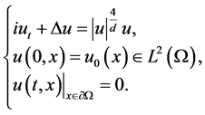 (1)
(1)
Here  and the initial data
  will only be required to the
  space.
This equation has Hamiltonian
 (2)
(2)
As (2) is preserved by (1), we shall refer to it as the mass and often write  or M for
 .
.
H. Brezis and T. Gallouet [1] considered that  in
in ,
,  , the nonlinear Schrödinger equation in
  of a bounded domain or an exterior domain of
 ![]() with Dirichlet boundary conditions. In [2] , N. Burq, P. Gérard and N. Tzvetkov described nonlinear Schrödinger equations in exterior domains. In [3] [4] , R. Killip, M. Visan and X. Zhang considered the defocusing energy-critical nonlinear Schrödinger equation and the focusing cubic nonlinear Schrödinger equation in the exterior domain
with Dirichlet boundary conditions. In [2] , N. Burq, P. Gérard and N. Tzvetkov described nonlinear Schrödinger equations in exterior domains. In [3] [4] , R. Killip, M. Visan and X. Zhang considered the defocusing energy-critical nonlinear Schrödinger equation and the focusing cubic nonlinear Schrödinger equation in the exterior domain ![]() of a smooth, compact, strictly convex obstacle in
of a smooth, compact, strictly convex obstacle in ![]() with Dirichlet boundary conditions, respectively.
with Dirichlet boundary conditions, respectively.
In [5] , T. Tao and M. Visan established stability of energy-critical nonlinear Schrödinger equations in![]() . However, we established stability of mass-critical nonlinear Schrödinger equations in the exterior domain
. However, we established stability of mass-critical nonlinear Schrödinger equations in the exterior domain ![]() in
in ![]() (
(![]() ).
).
Throughout this paper, we restrict ourselves to the following notion of solution.
Definition 1 (solution). Let I be a time interval containing zero, a function ![]() is called a solution to (1) if it lies in the class
is called a solution to (1) if it lies in the class ![]() for any compact interval
for any compact interval![]() , and it satisfies the Duhamel formula
, and it satisfies the Duhamel formula
![]() (3)
(3)
for all![]() . The interval I is said to be maximal if the solution cannot be extended beyond I. We say u is a global solution if
. The interval I is said to be maximal if the solution cannot be extended beyond I. We say u is a global solution if![]() .
.
In this formulation, the Dirichlet boundary condition is enforced through the appearance of the linear propagator associated to the Dirichlet Laplacian.
Our stability theorem concerns mass-critical stability in ![]() for the initial-value problem associated to the Equation (1).
for the initial-value problem associated to the Equation (1).
Theorem 2 (Stability theorem). Suppose![]() , I is a compact interval and let
, I is a compact interval and let ![]() be an approximate solution to
be an approximate solution to
![]() (4)
(4)
in the sense that
![]() (5)
(5)
for some function e.
Assume that
![]() (6)
(6)
![]() (7)
(7)
for some positive constants M and L.
Let ![]() and
and ![]() obey
obey
![]() (8)
(8)
for some![]() . Moreover, assume the smallness conditions
. Moreover, assume the smallness conditions
![]() (9)
(9)
![]() (10)
(10)
for some![]() , where
, where ![]() is a small constant.
is a small constant.
Then, there exists a solution u to
![]() (11)
(11)
on ![]() with initial data
with initial data ![]() at time
at time ![]() satisfying
satisfying
![]() (12)
(12)
![]() (13)
(13)
![]() . (14)
. (14)
The rest of the paper is organized as follows. In Section 2, we introduce our notations and state some previous results. In Section 3, we finally prove Theorem 2, except for proving a lemma about approximate solutions.
2. Preliminaries and Notations
In this section we summarize some our notations and collect some lemmas that are used in the rest of the paper.
We write ![]() to signify that there is a constant
to signify that there is a constant ![]() such that
such that![]() . We use the notation
. We use the notation ![]() whenever
whenever![]() . If the constant C involved has some explicit dependency, we emphasize it by a subscript. Thus
. If the constant C involved has some explicit dependency, we emphasize it by a subscript. Thus ![]() means that
means that ![]() for some constant
for some constant ![]() depending on u. We write
depending on u. We write ![]() for the nonlinearity in (1).
for the nonlinearity in (1).
We define that for some![]() ,
,
![]()
![]()
We also define ![]() to be the space dual to
to be the space dual to ![]() with appropriate norm.
with appropriate norm.
With these notations, the Strichartz estimates read as follows:
Theorem 3 (Strichartz estimates [3] [6] ). Let ![]() be a time interval and let
be a time interval and let![]() , then the solution
, then the solution ![]() to
to
![]()
satisfies
![]()
Proposition 4 (Local well-posedness). Given![]() , there exists
, there exists ![]() such that if
such that if ![]() and
and
![]()
on some interval![]() ,
, ![]() , then there exists a unique solution
, then there exists a unique solution ![]() of (1) satisfying
of (1) satisfying![]() . Besides,
. Besides,
![]()
The quantities ![]() defined in (2) are conserved on I.
defined in (2) are conserved on I.
3. Proof of Theorem 2
We need the following lemma to prove this theorem.
Lemma 1. Let I be a compact interval and let ![]() be an approximate solution to
be an approximate solution to
![]() (15)
(15)
in the sense that
![]() (16)
(16)
for some function e.
Assume that
![]() (17)
(17)
for some positive constant M.
Let ![]() and
and ![]() be such that
be such that
![]() (18)
(18)
for some![]() .
.
Assume also the smallness conditions
![]() (19)
(19)
![]() (20)
(20)
![]() (21)
(21)
for some![]() , where
, where ![]() is a small constant.
is a small constant.
Then, there exists a solution u to
![]() (22)
(22)
on ![]() with initial data
with initial data ![]() at
at ![]() satisfying
satisfying
![]() (23)
(23)
![]() (24)
(24)
![]() (25)
(25)
![]() . (26)
. (26)
Proof of Lemma 1. By symmetry, we may assume![]() . Let
. Let![]() , then w satisfies the following problem
, then w satisfies the following problem
![]()
where![]() .
.
For![]() , we define
, we define
![]()
By (19),
![]() (27)
(27)
On the other hand, by Strichartz, (20), (21), we get
![]() (28)
(28)
Combining (27) and (28), we obtain
![]()
By bootstrapping, we see if ![]() is taken sufficiently small,
is taken sufficiently small,
![]()
which implies (26).
Using (26) and (28), we see (23).
Moreover, by Strichartz, (18), (21) and (26),
![]()
which establishes (24) for ![]() sufficiently small.
sufficiently small.
To show (25), we use Strichartz, (17), (18), (26), (19),
![]()
Choosing ![]() sufficiently small, this finishes the proof of the lemma. W
sufficiently small, this finishes the proof of the lemma. W
We now turn to the proof of stability theorem.
Proof of Theorem 2. We now subdivide I into ![]() subintervals
subintervals
![]() ,
, ![]() , such that
, such that
![]()
where ![]() as in the lemma.
as in the lemma.
We need to replace ![]() by
by ![]() as the mass of the difference
as the mass of the difference ![]() might grow slightly in time.
might grow slightly in time.
By choosing ![]() sufficiently small depending on J, M and
sufficiently small depending on J, M and![]() , we can apply the lemma to obtain for each j and all
, we can apply the lemma to obtain for each j and all![]() ,
,
![]()
![]()
![]()
![]()
provided we can show that analogues of (8) and (9) hold with ![]() replaced by
replaced by![]() .
.
In order to verify this, we use an inductive argument.
By Strichartz, (8), (10) and the inductive hypothesis,
![]()
Similarly, by Strichartz, (9), (10) and the inductive hypothesis, we see
![]()
so we see
![]()
Choosing ![]() sufficiently small depending on J, M and
sufficiently small depending on J, M and![]() , we can guarantee that the hypotheses of the lemma continue to hold as j varies. W
, we can guarantee that the hypotheses of the lemma continue to hold as j varies. W
4. Conclusion
In this paper, we consider a mass-critical stability of the defocusing mass-critical nonlinear Schrödinger equation. Then we prove two different types of perturbation to show the stability of nonlinear Schrödinger equation.
Acknowledgements
The research of Guangqing Zhang has been partially supported by the NSF grant of China (No. 51509073) and also “The Fundamental Research Funds for the Central Universities” (No. 2014B14214). The author would like to thank his tutor Zhen Hu for helpful conversations. The author also thanks the referees for their time and comments.