Noise-Dependent Stability of the Synchronized State in a Coupled System of Active Rotators ()
1. Introduction
Networks of coupled nonlinear oscillators provide useful model systems for the study of a variety of phenomena in physics and biology [1]. Among many others, examples from physics include solid-state lasers [2] and coupled Josephson junctions [3,4]. In biology, the central nervous system can be described as a complex network of oscillators [5], and cultured networks of heart cells are examples of biological structures with strong nearest-neighbor coupling [6]. In particular, the emergence of synchrony in such networks [7,8] has received increased attention in recent years.
Disorder and noise in physical systems usually tend to destroy spatial and temporal regularity. However, in nonlinear systems, often the opposite effect is found and intrinsically noisy processes, such as thermal fluctuations or mechanically randomized scattering, lead to surprisingly ordered patterns [9]. For instance, arrays of coupled oscillators can be synchronized by randomizing the phases of their driving forces [10,11]. Synchronization in these systems is caused by the interactions between the elements and results in the emergence of collective modes. It has been shown to be a fundamental mechanism of self-organization and structure formation in systems of coupled oscillators [12]. Biological systems of neurons are subject to different sources of noise, such as synaptic noise [13] or channel noise [14]. In particular, sensory neurons are notoriously noisy. Therefore, the question arises how stochastic influences affect the functioning of biological systems. Especially interesting are scenarios in which noise enhances performance. In the case of stochastic resonance [15], e.g., noise can improve the ability of a system to transfer information reliably, and the presence of this phenomenon in neural systems has been investigated [16,17]. Furthermore, numerous studies have addressed the effect of noise on the dynamics of limit cycle systems [18-23].
Small neural circuits composed of two or three neurons form the basic feedback mechanisms involved in the regulation of neural activity [24]. They can display oscillatory activity [25,26] and serve as central pattern generators involved in motor control [27]. Here, we consider a system of two limit cycle oscillators with repulsive coupling. We investigate the influence of the noise and the coupling strength on the dynamics of the system. We distinguish between two different classes of dynamics, a synchronized state, in which the joint probability density of the oscillator phases is characterized by a single-hump shape, and a desynchronized state. The single-hump shaped distribution of the oscillator phases has been modeled by a Gaussian distribution [28,12], and systems consisting of a large number of oscillators were analyzed by examining the resulting dynamics for the mean of the oscillator phases [20]. In contrast, the simplicity of our two oscillator system allows us to obtain the stationary probability density function for the full system both numerically and analytically. We show that the probability distribution of the oscillator phases has the single-hump shape only for weak coupling, whereas it deviates from this shape for strong coupling. We evaluate the coupling strength at which the transition between the two forms of the probability distribution occurs as a function of the noise intensity.
In Section 2, we introduce the Kuramoto model for excitable systems. Under the influence of noise, the dynamics of the limit cycle oscillators are described by a stochastic differential equation (SDE), and we state the Fokker-Planck equation for the system. In Section 3, we consider a single active rotator driven by noise and derive its mean angular frequency from the stationary solution to the Fokker-Planck equation. We compare our analytical results with Monte-Carlo simulations of the corresponding SDE. In Section 4, we consider two coupled deterministic rotators and perform a bifurcation analysis of the system. We show that the system possesses a fixed point that is stable for small coupling strengths but loses its stability when the coupling is increased. For some range of the coupling strength, the stable fixed point and a stable limit cycle coexist. In Section 5, we consider two coupled active rotators under uncorrelated stochastic influences. In Section 5.1, we solve the Fokker-Planck equation of the system numerically and show that the shape of the probability distribution undergoes a characteristic change, corresponding to the transition from a synchronized to a desynchronized state, as coupling is increased. We evaluate the boundary between the synchronous and the asynchronous regime through a Fourier expansion approach in Section 5.2. A summary concludes the paper in Section 6.
2. Excitable Systems and the Kuramoto Model
Neurons can display a wide range of behavior to different stimuli and numerous models exist to describe neuronal dynamics. A common feature of both biological and model neurons is that sufficiently strong input causes them to fire periodically; the neuron displays oscillatory activity. For subthreshold inputs, on the other hand, the neuron is quiescent. When a subthreshold input is combined with a noisy input, however, the neuron will be pushed above threshold from time to time and fire spikes in a stochastic manner. In this regime, the neuron acts as an excitable element. In general, an excitable system possesses a stable equilibrium point from which it can temporarily depart by a large excursion through its phase space when it receives a stimulus of sufficient strength [22]. Besides neurons, chemical reactions, lasers, models of blood clotting, and cardiac tissues all display excitable dynamics [29-33]. Pulse propagation, spiral waves, spatial and temporal chaos, and synchronization have been studied in these systems [34-37].
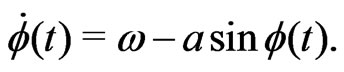
The phase dynamics of an active rotator without interaction and random forces can be described by the model developed by Kuramoto and coworkers [38,39]:
 (1)
(1)
To obtain the case of the excitable system with one stationary point, one chooses the parameter . When we have n coupled identical oscillators, subject to stochastic influences, the model is described by the Langevin Equation [23]
 (2)
(2)
Here, we take the  to be uncorrelated Gaussian white noise, i.e.
 ,
, . We will concentrate on the simplest case, namely that the coupling functions
  are sin-functions multiplied by a coupling constant
 , i.e.,
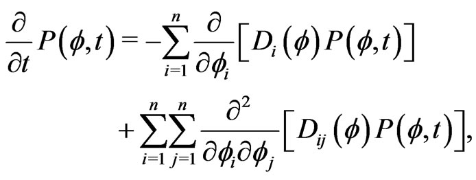
 . Then, the dynamical evolution of the system's probability density function
  is described by the Fokker-Planck equation
 (3)
(3)
where in our case the drift terms read
 (4)
(4)
and the diffusion terms are given by
 (5)
(5)
Since the angle variables  describe the phases of the oscillators, the probability density function must satisfy the periodic boundary conditions
 (6)
(6)
Furthermore, the normalization condition for the probability density reads
 (7)
(7)
3. Single-Rotator System
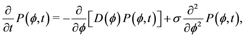
We first exam a single rotator subject to a noisy input and, following Ref. [40], calculate the mean frequency of oscillations as a function of the noise level. In this case, the Fokker-Planck Equation (3) reads
 (8)
(8)
with
 (9)
(9)
We can thus write the drift term as the negative gradient of a potential, 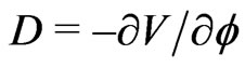 , with the potential given by
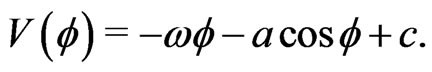 (10)
(10)
Introducing the probability current
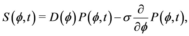 (11)
(11)
the Fokker-Planck equation takes the form of a continuity equation,
 (12)
(12)
We now look for a stationary solution of the form ,
, . In this case, we conclude from (12) that the derivative of the probability current with respect to
  must vanish, and we have to solve
 (13)
(13)
The constant probability current S is related to the mean drift velocity, i.e., the mean angular frequency of the active rotator system according to . The solution to the ordinary differential Equation (13) is given by
 (14)
(14)
The integration constant in (10) can thus be absorbed into the constant C in (14), and the two free constants S and C are determined by the periodicity and normalization conditions (6) and (7). These two conditions can be written in matrix form as
 (15)
(15)
Denoting the determinant of the  matrix in the last expression as det, the constants C and S are given by
 (16)
(16)
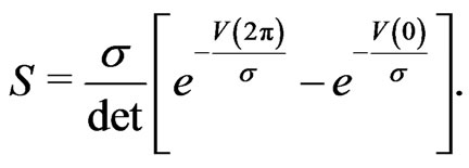 (17)
(17)
Specializing to the potential of the active rotator (10), we obtain
 (18)
(18)
Note that in the limit  the integrand in the denominator approaches one, and
  converges to
 . To obtain the leading order behavior of
  in the limit of small noise, we approximate the denominator using Laplace's method described in Ref. [41]. According to Laplace's method the asymptotic behavior of the integral
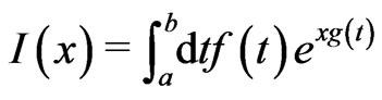 (19)
(19)
as  is given by
 (20)
(20)
Here, it is assumed that  has a maximum at
  with
with  and that
  and
and . We first apply Laplace's method to the inner integral in the denominator of (18), which we denote as
 . The function
  has a maximum inside the interval
  at
at
 (21)
(21)
Using (20) we thus obtain for 
 (22)
(22)
The argument of the exponential function in the last identity can be simplified to
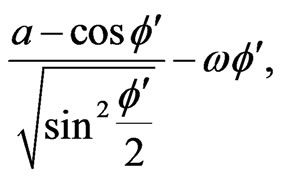 (23)
(23)
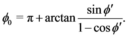
whose maximum within the interval  is at
is at
 (24)
(24)
Using this and applying (20) to the intermediate result (22), we obtain
 (25)
(25)
The leading asymptotic behavior of  as
as  is then given by
 (26)
(26)
Figure 1 shows the mean angular frequency  as a function of the noise level
 . The evaluation of the analytical expression (18) yields results that are in good agreement with Monte-Carlo simulations of the Langevin Equation (2). Furthermore, the asymptotic expansion (26) is in excellent agreement with numerical evaluations of (18) for small noise.
4. Deterministic Two-Rotator System
We next turn to a system of two coupled active rotators, where we first consider the deterministic case, i.e. . In particular, we are interested in rotators with repulsive coupling, i.e. we consider the case
 . Introducing the center of mass and difference coordinates
  and
and , the set of Equations (2) takes the form

 (27)
(27)
The system has a trivial stationary point at ,
,  , whose stability we analyze by linearizing the system (27). Writing
 ,
,  we obtain to first order
 (28)
(28)
The real parts of the eigenvalues of the  matrix on the right-hand side of the last identity determine the stability of the fixed point
 . Under the assumption
  the first eigenvalue
  is always real and negative. The second eigenvalue
 is also always real; for small coupling it is negative, but when the sum of the coupling strengths
  increases it becomes positive and the fixed point
  loses its stability in, as it turns out, a subcritical pitchfork bifurcation. Further fixed points of the system can be determined and turn out to be unstable for all values of the coupling strengths. In the case
  they are given by
 (29)
(29)
Figure 2(a) shows a bifurcation diagram of the system. For small coupling strength, the system does not display oscillatory behavior. When the coupling strength is increased above a critical value, a stable limit cycle emerges
from a homoclinic orbit. For a small range of coupling strengths, the stable fixed point coexists with the stable limit cycle. In this case, it depends on the initial conditions whether the system will converge toward the fixed point  or the limit cycle. Figure 2(b) shows the attractors for fixed point and limit cycle dynamics in the
  -plane for
 . In the strong-coupling limit, the minimum and maximum of
  in Figure 2(a) both converge toward
 . Thus, the system approaches antisynchronous oscillatory dynamics, where
  and
and  are phase shifted by
  while their sum increases constantly.
5. Stochastic Two-Rotator System
We now consider the coupled two-rotator system in the case where both rotators receive uncorrelated stochastic driving. The temporal evolution of the probability density of this system is given by the Fokker-Planck Equation (3) with the drift and diffusion coefficients (4) and (5).
5.1. Numerical Results
First, we investigate the stationary solution to the Fokker-Planck equation numerically. To this end, we numerically solve the partial differential Equation (3) under the periodic boundary conditions (6) for the homogeneous initial condition  and observe that the solution converges to the stationary solu-
tion after some time. Figure 3 shows the stationary solution in the coordinates  and
and  for two different values of the coupling strength. We find that, depending on the strength of the noise and coupling, two different characteristic forms of the stationary solution exist. In the case shown in Figure 3(a) the probability density is peaked around the stable fixed point of the deterministic two-rotator system
 . In Figure 3(b), the peak at the fixed point
  is much less pronounced. Furthermore, if we consider the probability distribution for
 , i.e., at the edge of the region shown in Figure 3, we see that the probability distribution is not given by one central hump anymore. In order to distinguish between the two different scenarios in a quantitative way, we consider the marginal stationary probability density
 (30)
(30)
Figure 4 shows this quantity for one level of the noise intensity  and for different coupling strengths. For weak coupling,
  has a pronounced maximum at
 . For increasing coupling strengths, this maximum decreases and eventually turns into a minimum. We can thus classify the system dynamics as synchronized or desynchronized according to the sign of the second derivative of
  at the origin and can label the
  -w plane accordingly. In the next section, we calculate the phase boundary between the synchronized and desynchronized regime through a Fourier expansion approach.