New Asymptotical Stability and Uniformly Asymptotical Stability Theorems for Nonautonomous Difference Equations ()
Received 15 April 2016; accepted 4 June 2016; published 7 June 2016

1. Introduction
Difference equations usually describe the evolution of certain phenomena over the course of time. These equations occur in biology, economics, psychology, sociology, and other fields. In addition, difference equations also appear in the study of discretization methods for differential equations. Realizing that most of the problems that arise in practice are nonlinear and mostly unsolvable, the qualitative behaviors of solutions without actually computing them are of vital importance in application process. The stability property of an equilibrium is the very important qualitative behavior for difference equations. The most powerful method for studying the stability property is Liapunov’s second method or Liapunov’s direct method. The main advantage of this method is that the stability can be obtained without any prior knowledge of the solutions. In 1892, the Russian mathematician A.M. Liapunov introduced the method for investigating the stability of nonlinear differential equations. According to the method, he put forward Liapunov stability theorem, Liapunov asymptotical stability theorem and Liapunov unstable theorem, which have been known as the fundamental theorems of stability. Utilizing these fundamental theorems of stability, many authors have investigated the stability of some specific differential systems [1] - [9] .
We know that several results in the theory of difference equations have been obtained as more or less natural discrete analogues of corresponding results of differential equations, so Liapunov’s direct method is much more useful for difference equations. Actually, some authors have utilized the methods for difference equations successfully [10] - [20] . Using the method, S. Elaydi [10] and J.P. Lasalle [11] gave the classical Liapunov stability theorem for autonomous difference equations. In [12] [13] , the authors extended the technique to generalized nonautonomous difference equations and put forward the classical Liapunov stability theorem for nonautonomous difference equations. In [14] - [17] , the direct approach was extended to some special delay difference systems to investigate the stability properties. In [18] - [20] , how to construct Liapunov function for difference system or hybrid time-varying system was exploited.
Consider the following nonautonomous difference system
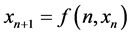 (1.1)
(1.1)
where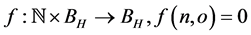 ,
,  is continuous in x and
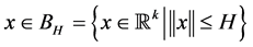 . As shown in [12] [13] , using Liapunov’s direct method to study the asymptotical stability of the zero solution of system (1.1) relies on the existence of a positive definite Liapunov function
  which has indefinitely small upper bound and whose variation
  along the solution of system (1.1) is negative definite.
Sometimes it is not easy to determine the positive definite Liapunov function for a given equations in applications. If we further require that the function has indefinitely small upper bound besides its negative definite variation, the work would become more difficult to do. In this paper, we weaken the Liapunov function to positive definite and also weaken the negative definite variation to semi-negative definite on orbits of Equations (1.1), then we put forward a new Liapunov asymptotical stability theorem for difference Equations (1.1) by adding to extra conditions on the variation. Subsequently, provided that all the conditions of our new asymptotical stability theorem are satisfied, we obtain a new uniformly asymptotical stability theorem of nonautonomous difference equations if the Liapunov function has an indefinitely small upper bound.
2. Some Lemmas
In this section, we introduce the following lemmas, which play a key role in obtaining our results.
Lemma 1 Suppose that there exists a function  satisfying the following conditions:
(i)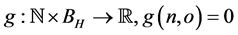 ,
,  is
is  with respect to the second argument x,
(ii) the sequence , and
, and
(iii)  exists.
Then, there exists a positive integer sequence  with
with  as
as  such that
![]() .
.
Proof. We first prove that for arbitrary constant ![]() there exists a sufficient large integer
there exists a sufficient large integer ![]() for every positive integer
for every positive integer ![]() such that
such that
![]() (2.1)
(2.1)
Suppose that this conclusion of inequality (2.1) does not hold, then there exist ![]() such that for arbitrary
such that for arbitrary ![]() there exists a positive integer
there exists a positive integer ![]() such that
such that
![]() (2.2)
(2.2)
By the continuity of![]() , we obtain that either
, we obtain that either ![]() or
or![]() . Without loss of generality, we only consider the first case. For the above
. Without loss of generality, we only consider the first case. For the above![]() , there exists a positive integer increasing sequence
, there exists a positive integer increasing sequence ![]() such that
such that ![]() for arbitrary
for arbitrary![]() . Let
. Let ![]() denote a constant. By the discrete analogue fundamental theorem of calculus [10] , we get
denote a constant. By the discrete analogue fundamental theorem of calculus [10] , we get
![]()
Note that ![]() is a positive integer increasing sequence and
is a positive integer increasing sequence and![]() , then the above inequality contradicts
, then the above inequality contradicts
to the exists of ![]() Therefore, the conclusion of (2.1) is proved.
Therefore, the conclusion of (2.1) is proved.
Denote ![]() with
with ![]() By the conclusion of (2.1), for each i, there exists a sufficiently large
By the conclusion of (2.1), for each i, there exists a sufficiently large
![]() such that
such that
![]() (2.3)
(2.3)
for each positive integer![]() . Then we can select special
. Then we can select special ![]() and construct an increase sequence
and construct an increase sequence
![]() . This implies
. This implies ![]() as
as ![]() and
and ![]()
Lemma 2 Assume that there exists a function ![]() satisfying the following conditions:
satisfying the following conditions:
(i)![]() ,
, ![]() is
is ![]() with respect to the second argument,
with respect to the second argument,
(ii) the sequence![]() , and
, and
(iii) ![]() exists.
exists.
Then, for each fixed r![]() , there exists a positive integer sequence
, there exists a positive integer sequence ![]() with
with ![]() as
as ![]() such that
such that
![]()
Proof. We first prove that for arbitrary constants ![]() there exists a sufficient large integer
there exists a sufficient large integer ![]() such that for every
such that for every ![]() there exists
there exists
![]() (2.4)
(2.4)
The case of ![]() is proved by (2.1) in the proof of Lemma 2.1. Suppose that inequality (2.4) holds in the case of
is proved by (2.1) in the proof of Lemma 2.1. Suppose that inequality (2.4) holds in the case of ![]()
![]() but is not true in the case of r. Then there exist constants
but is not true in the case of r. Then there exist constants ![]() such that for arbi-
such that for arbi-
trary ![]() there exists a positive integer
there exists a positive integer ![]() such that
such that![]() . Similarly to the state-
. Similarly to the state-
ment below inequality (2.2), there exists a positive integer sequence ![]() such that
such that![]() .
.
Let ![]() denote the maximum integer not exceeding x and
denote the maximum integer not exceeding x and ![]() denote a constant. Same as above, without loss of generality, we only consider the case
denote a constant. Same as above, without loss of generality, we only consider the case![]() . By the discrete analogue fundamental theorem of calculus [10] , we get
. By the discrete analogue fundamental theorem of calculus [10] , we get
![]() (2.5)
(2.5)
where![]() .
.
![]() (2.6)
(2.6)
where![]() .
.
If ![]() and
and![]() , from inequality (2.5), we obtain
, from inequality (2.5), we obtain
![]() (2.7)
(2.7)
If ![]() and
and![]() , from inequality (2.6), we obtain
, from inequality (2.6), we obtain
![]() (2.8)
(2.8)
Inequalities (2.7) and (2.8) imply that
![]() (2.9)
(2.9)
Since ![]() as
as![]() , we select
, we select![]() . This leads to a contradiction because of the inductive assumption for (2.4) in the case of
. This leads to a contradiction because of the inductive assumption for (2.4) in the case of![]() . Therefore, the conclusion of (2.4) is proved.
. Therefore, the conclusion of (2.4) is proved.
Similarly to the second part of the proof of Lemma 2.1, for each r![]() , we can construct a sequence
, we can construct a sequence
![]() with
with ![]() as
as ![]() such that
such that ![]() This completes the proof of Lemma 2.2.
This completes the proof of Lemma 2.2.
According to Lemma 2.2 we prove the following result.
Lemma 3 Assume that there exists a function ![]() satisfying the following conditions:
satisfying the following conditions:
(i)![]() ,
, ![]() is
is ![]() and
and ![]() is uniformly continuous with respect to the second argument x,
is uniformly continuous with respect to the second argument x,
(ii) the sequence![]() , and
, and
(iii) ![]() exists.
exists.
Then, there exists a positive integer sequence ![]() with
with ![]() as
as ![]() such that
such that
![]() (2.10)
(2.10)
Proof. Let us first prove
![]() (2.11)
(2.11)
Suppose that this is not true. Then there exist a constant c > 0 and a strictly increasing integer sequence ![]()
such that ![]() as
as ![]() and
and![]() ,
,![]() . By the uniform continuity of
. By the uniform continuity of![]() , there exists a constant
, there exists a constant![]() , when
, when ![]() for any
for any![]() , then
, then![]() . From the above inequalities, we get
. From the above inequalities, we get![]() . This is a contradiction to (2.4). Then equation (2.11) is proved.
. This is a contradiction to (2.4). Then equation (2.11) is proved.
The result of (2.11) implies the boundedness of ![]() on
on![]() . It follows that
. It follows that ![]() is
is
uniformly continuous on the same domain. And as shown above, we obtain ![]() Then we see recursively that
Then we see recursively that
![]() (2.12)
(2.12)
On the other hand, by Lemma 2.2, there exists a sequence ![]() with
with ![]() as
as ![]() such that
such that
![]() (2.13)
(2.13)
From (2.12) and (2.13) we easily get (2.10). The proof of Lemma 2.3 is complete .
3. New Asymptotical Stability and Uniformly Asymptotical Stability Theorems
In this section, we propose and prove the new asymptotical stability and uniformly asymptotical stability theorems of system (1.1). First of all, we introduce a special class of function and then give the definition of positive definite function. Subsequently, we introduce the various stability notions of the equilibrium point ![]() of system (1.1). These definitions are very useful for obtaining our results besides the above Lemmas.
of system (1.1). These definitions are very useful for obtaining our results besides the above Lemmas.
Definition 1 A function ![]() is said to be class of K if it is continuous in
is said to be class of K if it is continuous in![]() , strictly increasing, and
, strictly increasing, and![]() .
.
Definition 2 The function ![]() is positive definite if there exists a function
is positive definite if there exists a function ![]() such that
such that
![]()
for all![]() .
.
Definition 3 Let ![]() be an initial condition of system (1.1) and
be an initial condition of system (1.1) and ![]() be a solution such that
be a solution such that![]() . The equilibrium point
. The equilibrium point ![]() of system (1.1) is said to be:
of system (1.1) is said to be:
(i) Stable if given ![]() and
and ![]() there exists
there exists ![]() such that
such that ![]() implies
implies
![]() for all
for all![]() , uniformly stable if
, uniformly stable if ![]() may be chosen in dependent of
may be chosen in dependent of![]() .
.
(ii) Attracting if there exists ![]() such that
such that ![]() implies
implies![]() , uni-
, uni-
formly attracting if the choice of ![]() is independent of
is independent of![]() .
.
(iii) Asymptotically stable if it is stable and attracting, and uniformly asymptotically stable if it is uniformly stable and uniformly attracting.
Theorem 1 Consider nonautonomous difference Equations (1.1), where ![]() is
is ![]() with respect to the second argument x and satisfies
with respect to the second argument x and satisfies![]() . Suppose that there exists a
. Suppose that there exists a ![]() positive definite function
positive definite function ![]() such that
such that
(i)![]() ,
,
(ii)![]() , where
, where![]() ,
,
(iii) ![]() is bounded on the set
is bounded on the set![]() ,
,
(iv)![]() , where the func- tion
, where the func- tion ![]() defined by Definition 1.
defined by Definition 1.
Then the zero solution of system (1.1) is asymptotically stable.
tion ![]() with
with ![]() satisfies
satisfies ![]()
By condition (ii) we know that ![]() is monotonically nonincreasing. Hence the
is monotonically nonincreasing. Hence the ![]() exists.
exists.
From condition (iii) we know that ![]() is bounded, which implies that
is bounded, which implies that ![]() is uniformly con- tinuous. According to Lemma 3, there exists a integer sequence
is uniformly con- tinuous. According to Lemma 3, there exists a integer sequence ![]() with
with ![]() as
as ![]() such that
such that
![]() (3.1)
(3.1)
According to the definition of function ![]() and Equation (3.1), we get
and Equation (3.1), we get![]() , which implies
, which implies
![]() (3.2)
(3.2)
Now we prove
![]() (3.3)
(3.3)
Suppose that (3.3) is not true. Then there exist a constant ![]() and an integer sequence
and an integer sequence ![]() with
with ![]() as
as ![]() such that
such that ![]()
![]() . Then, by the definition of positive definite
. Then, by the definition of positive definite ![]()
![]() (3.4)
(3.4)
On the other hand, by (3.2) there is an integer j such that![]() . This is because V is continuous with respect to the second argument and
. This is because V is continuous with respect to the second argument and ![]() Thus, by condition (ii),
Thus, by condition (ii), ![]() for all
for all![]() . Clear,
. Clear, ![]() for sufficiently large l such that
for sufficiently large l such that![]() , which contradicts to the definition of v given
, which contradicts to the definition of v given
by (3.4). Therefore, (3.3) is proved. According to Definition 3, we obtain that the zero solution of system (1.1) is asymptotically stable.
In addition to the hypotheses of Theorem 1, we can obtain that the zero solution of system (1.1) is uniformly asymptotically stable if ![]() has an indefinitely small upper bound as in the classical Liapunov asymptotical stability theorem of nonautonomous difference equations.
has an indefinitely small upper bound as in the classical Liapunov asymptotical stability theorem of nonautonomous difference equations.
Theorem 2 Provided that the hypotheses of Theorem 1 are satisfied, the zero solution of system (1.1) is uniformly asymptotically stable if positive definite function ![]() has an indefinitely small upper bound.
has an indefinitely small upper bound.
Proof. Since ![]() is positive definite and has an indefinitely small upper bound, there exist functions
is positive definite and has an indefinitely small upper bound, there exist functions
![]() such that
such that ![]() for all
for all![]() . For each
. For each![]() , there exists a
, there exists a
![]() such that
such that![]() . Denote
. Denote ![]() and
and![]() , then we have
, then we have ![]() for all
for all![]() . If
. If
this is not true, then there exists a ![]() such that
such that ![]() and
and ![]() imply
imply![]() . However,
. However,
![]() implies that
implies that ![]() for
for![]() . Then we obtain that
. Then we obtain that
![]()
This is a contradiction. Since all the conditions of Theorem 1 are satisfied, the zero solution of system (1.1) is
asymptotically stable. Therefore, for the above![]() ,
, ![]() , there exists
, there exists ![]() when
when![]() .
.
4. Example
In this section, we provide an example to illustrate the feasibility of our results.
Example 4.1. Consider the following difference equations
![]() (4.1)
(4.1)
where ![]() and
and![]() . Obviously,
. Obviously,
f is C1 with respect to ![]() on
on ![]() and satisfies
and satisfies ![]() Denote
Denote ![]() and
and![]() . This function which satisfies
. This function which satisfies ![]() is clearly positive definite on
is clearly positive definite on ![]() and is
and is ![]() along the solutions of system (4.1), and
along the solutions of system (4.1), and
![]() (4.2)
(4.2)
Moreover,
![]()
For ![]() and
and![]() , we obtain
, we obtain![]() , then the zero solution of system (1.1) is stable. At the same condition, we also get
, then the zero solution of system (1.1) is stable. At the same condition, we also get
![]()
Now, we calculate![]() . For
. For![]() , we have
, we have
![]()
Then we get![]() , which means that
, which means that ![]() is bounded on the set
is bounded on the set![]() . Now, we only need to verify the example whether satisfies condition (iv) of
. Now, we only need to verify the example whether satisfies condition (iv) of
Theorem (3.1). Denote![]() ,
,![]() . Then
. Then ![]() is a class of K function. From the above analysis, we obtain
is a class of K function. From the above analysis, we obtain
![]()
Then,
![]()
Thus condition (iv) of Theorem (3.1) is fulfilled. The zero solution of Example 4.1 is asymptotical stable. Inequation (4.2) implies that ![]() has an indefinitely small upper bound. Then the zero solution of Example 4.1 is also uniformly asymptotically stable.
has an indefinitely small upper bound. Then the zero solution of Example 4.1 is also uniformly asymptotically stable.
We also can utilize Polar coordinate transformation to prove the above conclusion. Let ![]() and
and![]() , then system (4.1) transforms the following form:
, then system (4.1) transforms the following form:
![]() (4.3)
(4.3)
The square of the first equation adding the square of the second equation in system (4.3) yields
![]()
Denote ![]() and we get
and we get ![]() Under the conditions of
Under the conditions of ![]() and
and![]() , we obtain
, we obtain ![]() and
and![]() . By Definition 3, we obtain the zero solution of the
. By Definition 3, we obtain the zero solution of the
original system (4.1) is asymptotical stable and uniformly asymptotically stable. This confirm the correctness of utilizing Theorem 3.1 and Theorem 3.2 to judge Example 4.1.
Funding
This work was supported by the National Natural Science Foundation of China (Grant No.31170338), the General Project of Educational Commission in Sichuan Province (Grant No.16ZB0357) and the Major Project of Sichuan University of Arts and Science (Grant No.2014Z005Z).
NOTES
![]()
*Corresponding author.