A Novel Triangular Chaotic Map (TCM) with Full Intensive Chaotic Population Based on Logistic Map ()
Received 27 November 2015; accepted 28 December 2015; published 31 December 2015

1. Introduction
Over the last few years, many researchers have studied chaos theory in several fields, such as electronic systems, fluid dynamics, lasers, weather and climate [1] -[5] . Chaos theory is implementing today in many different fields of studies such as: engineering, computer science, mathematics, physics, geology, microbiology, biology, economics, finance, algorithmic trading, meteorology, philosophy, politics, population dynamics, psychology, and robotics [6] . Moreover, Chaos theory has attracted the cryptography field due to its characteristics, such as its deterministic nature, unpredictability, random-look nature and its sensitivity to initial value [7] .
Cryptographers have utilized dynamic chaotic maps to develop new cryptographic primitives by exploiting chaotic maps, such as logistic maps, Henon maps, and Tent maps. There are similarities and differences between cryptography algorithms and chaotic maps [8] . The parameters in chaotic maps are meaningful, if they are real numbers, which can be used in the cryptographic algorithms as encryption and decryption keys. Chaotic systems are sensitive to any change or changes in the initial condition(s) and are unpredictable in the long term, thus representing the diffusion in cryptographic encryption algorithms. Iterations of a chaotic map lead to the spread- ing of the initial region over the entire phase space, and this can be achieved in cryptographic algorithms by designing the algorithm based on rounds. The main difference between chaos and cryptography is that encryption transformations are defined on finite sets, whereas chaos has meaning only in real numbers.
Since 1990, many studies on digital chaotic cryptography have been proposed to provide secure communications based on chaotic maps including chaotic block ciphers [9] -[34] , chaotic cryptography hash functions [7] [31] [35] - [49] , and chaotic pseudorandom number generators [11] [50] - [65] . In general, chaos theory has been proved a secure algorithm against known cryptanalysis techniques. Recently, various studies have been conducted on chaotic cryptographic algorithms [7] [66] - [87] . Some of the proposed chaotic cryptographic algorithms that have been analysed have had weak internal designs and incorrect exploitation of chaotic maps. In this research, we propose novel triangular chaotic map.
The rest of this research paper is organized as follows. Section 2 introduces chaos theory. The details of chaotic maps are discussed in Section 3. Section 4 describes details of Logistic map and Lyapunov exponent. In Section 5, details of the new Triangular Chaotic map are given. Finally, the conclusion is given in Section 6.
2. Chaos Theory
Chaos is derived from a Greek word “Xαos”, meaning a state without order or predictability [2] . A chaotic system is a simple, non-linear, dynamical, and deterministic system that shows completely unpredictable behaviour and appears random [88] . Moreover, it is a deterministic system with great sensitivity to initial conditions, such that a computer system can give an amazingly different result when the value of an input parameter is changed. On the other hand, in classical science small changes in an initial value might generate small differences in the result [89] [90] . A system is called a chaotic system if it is sensitive to initial conditions, topology mix, and if periodic orbits are dense.
According to Alligood et al. (1996), a dynamical system contains all the possible states and regulations that control the next state from the current state. On the other hand, the deterministic regulations are those that determine the current state uniquely from the previous states, whereas there is always a mathematical equation to determine the system evolution [91] . From the previous definitions of deterministic and dynamical systems, we cannot say that the randomness is not allowed. The bifurcation in dynamic differential equation changes the number of solutions as the parameters is changed [92] .
In 1890, Poincaré published his article [89] (on the equations of the dynamics and the three-body problem) of 270 pages, which simplified the way of looking at the complicated continuous trajectories from differential equations [2] . Then, in 1898, Hadamard observed the sensitivity to initial conditions and unpredictability of special systems, calling this the geodesic flow [2] . Later, in 1908, Poincaré noted that chaos sensitivity depends on initial conditions and gives unpredictable results [90] [93] . Later on, Edward Lorenz (1963) examined chaos theory and described a simple mathematical model of weather prediction [91] . Lorenz’s model was the first numerical model to detect chaos in a non-linear dynamical system [3] [94] . Lorenz’s findings were very interesting in that some equations rise to some surprisingly complex behaviour and chaos behaviour dependent on the initial condition [2] . In 1975, Li and Yorke were the first to introduce the word ‘chaos’ into mathematical literature, where system results appear random [1] - [5] [95] [96] .
Chaotic maps have been the subject of an extremely active research area due to their characteristics, such as sensitivity to the initial value, complex behaviour, and completely deterministic nature. The chaotic behaviour can be observed in many different systems, such as electronic systems, fluid dynamics, lasers, weather, climate and economics [2] [88] [89] [97] . Our intuition tells us that a small change in input parameters should give a small change in output, but chaotic systems show us that this is not necessarily the case. Usually, chaotic maps define infinitely large fields of real numbers. The most important characteristics of chaotic systems are as follows:
1. Apparently random behaviour but completely deterministic: The behaviour of chaotic systems seems to be random but actually it is purely deterministic. Hence, if we run the chaotic system many times with the same initial value, we will obtain the same set of output values. Furthermore, the chaotic systems are dynamical systems that are described by differential equations or iterative mappings, and the next state is specified from the previous state (see Equation 3-1 [5] [98] [99] ).
 (1)
(1)
2. Sensitivity dependence on the initial conditions (The state from which the system starts): Dynamical systems evolve completely differently over time with slight changes in the initial state [88] [90] .
3. Unpredictable (difficult or impossible to predict the behaviour in the long term): In chaotic maps, even if one knows the current state of the chaotic system it is useless trying to predict the next state of the system. In other words, it is very difficult to predict the future states of the chaotic system in the long term [89] [100] .
3. Chaotic Maps
According to Alligood et al. (1996), a chaotic map is a function of its domain and range in the same space, and the starting point of the trajectory is called the initial value (condition) [101] . Chaotic dynamics have a unique attribute that can be seen clearly by imagining the system starting twice with slightly different initial conditions [102] . Chaos theory attempts to explain the result of a system that is sensitive to initial conditions, complex, and shows unpredictable behaviour. Chaotic dynamical systems increase communication security with higher dimensions and more than one positive Lyapunov exponent [91] . A Lyapunov exponent is used to help select the initial parameters of chaotic maps that fall in chaotic areas. A chaotic system exhibits some chaotic behaviour and often occurs in the study of dynamical systems. In the following subsections, we will give a brief induction to some chaotic systems: Logistic map, Lorenz attractors, Rossler attractors, Henon map, Tent map, and Piecewise linear chaotic map.
3.1. Logistic Map
In 1845, Pierre Verhulst proposed a logistic map, which is a simple non-linear dynamical map. A logistic map is one of the most popular and simplest chaotic maps [103] . Logistic maps became very popular after they were exploited in 1979 by the biologist Robert M. May [89] . The logistic map is a polynomial mapping, a complex chaotic system, the behaviour of which can arise from very simple non-linear dynamical equations, as shown in Figure 1 [104] . The logistic map equation is written as:
 (2)
(2)
where  is a number between zero and one,
  represents the initial population, and r is a positive number between zero and four.
![]()
Figure 1. Bifurcation diagram of the Logistic map [105] .
The logistic map is one of the simplest chaotic maps; it is highly sensitive to change in its parameter value, where a different value of the parameter r will give a different map f [89] . Its transformation function is F:  which is defined in the above equation. From the onset of chaos, a seemingly random jumble of dots, the behaviour of the logistic map depends mainly on the values of two variables (r, x0); by changing one or both variables’ values we can observe different logistic map behaviours. The population of a logistic map will die out if the value of r is between 0 and 1, and the population will be quickly stabilized on the value
  if the value of r is between 1 and 3 [89] . Then, the population will oscillate between two values if the value of parameter r is between 3 and 3.45. After that, with values of parameter r between 3.45 and 4 the periodic fluctuation becomes significantly more complicated. Finally, most of the values after 3.57 show chaotic behaviour.
In the logistic map , the function result depends on the value of parameter r, where different values of r will give quite different pictures. We can note that g(x1) = x2 and g(x2) = x1, that mean
  and
and . According to Alligood et al. (1996) the periodic fluctuation between x1, x2 is steady and attracts orbits (trajectories). Therefore, there are a minimum number of iterations of the orbit to repeat the point. There are obvious differences between the behaviour of the exponential model and the logistic model’s behaviour. To show the difference between the two functions, we take an example of the exponential function
  and an example of logistic function
 ; the initial value for both functions is 0.0090, and we then calculate the population for n = 0, 1, 2,
  , 10 resulting in an accuracy of five decimal places. We can notice that the output values of the exponential function are always increasing as time progresses, while the output values of the logistic function are fluctuating with a finite limited size between zero and one [88] [89] [93] .
3.2. Lorenz Attractor
The Lorenz attractor is one of the most popular three-dimensional chaotic attractors; it was examined and introduced by Edward Lorenz in 1963 [2] . He showed that a small change in the initial conditions of a weather model could give large differences in the resulting weather. This means that a slight difference in the initial condition will affect the output of the whole system, which is called sensitive dependence to the initial conditions. The non-linear dynamical system is sensitive to the initial value and is related to the system’s periodic behaviour [90] . Lorenz’s dynamic system presents a chaotic attractor, whereas the word chaos is often used to describe the complicated manner of non-linear dynamical systems [106] . Chaos theory generates apparently random behaviour but at the same time is completely deterministic, as shown in Figure 2. The Lorenz attractor is defined as follows:
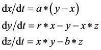 (3)
(3)
![]()
Figure 2. A plot of the trajectory of the Lorenz system, (modified from [107] )
3.3. Rossler Attractors
In 1976 [88] [89] , O. Rossler created a chaotic attractor with a simple set of non-linear differential equations [88] . Rossler attempted to write the simplest dynamical system that exhibited the characteristics of a chaotic system [89] [108] . The Rossler attractor was the first widely-known chaotic attractor from a set of differential equations; defined by a set of three non-linear differential equations, the system exhibits a strange attractor for a = b = 0.2 and c = 5.7 (see Equation (4)) [108] . The Rossler attractor is a rather nice but not famous attractor, which draws a nifty picture of a non-linear three-dimensional deterministic dynamical system, as shown in Figure 3.
![]() (4)
(4)
A, B, and C are constants.
3.4. Henon Attractors
The Henon map is one of the dynamical systems that exhibit chaotic behaviours. The Henon map is defined by two equations; the map depends on two parameters a, b, and the system exhibits a strange attractor for a = 1.4 and b = 0.3 (see Equation (5)). A Henon map takes one point (x, y) and maps this point to a new point in the plane, as shown in Figure 4 [108] .
![]() (5)
(5)
3.5. Tent Map
A Tent map is an iterated function of a dynamical system that exhibits chaotic behaviours (orbits) and is governed by Equation (6). It has a similar shape to the logistic map shape with a corner (Figure 5 and Figure 6)
![]()
Figure 4. Henon attractor for a = 1.4 and b = 0.3 [89] .
![]()
Figure 5. Bifurcation diagram for the tent map [110] .
[109] . The Tent map exhibits the Lyapunov exponents on the unit interval ![]() and
and![]() . It is a simple one-dimensional map generating periodic chaotic behaviour similar to a logistic map.
. It is a simple one-dimensional map generating periodic chaotic behaviour similar to a logistic map.
![]() (6)
(6)
3.6. Piecewise Linear Chaotic Maps
Piecewise linear chaotic maps (PWLCMs) are simple non-linear dynamical systems with large positive Lyapunov exponents. In [111] , they are shown to have several brilliant chaotic properties that can be exploited in chaotic cryptographic algorithms. PWLCM has perfect behaviour and high dynamical properties such as invariant distribution, auto-correlation function, periodicity, large positive Lyapunov exponent, and mixing property [112] . Iterations of PWLCM with initial value and control parameters generate a sequence of real numbers between 0 and 1, which is called an orbit. A large positive Lyapunov exponent means that the system shows chaotic behaviour over large orbits [110] . The periodicity property indicates that the system behaviour is average over time and space. Correlation functions are a very important test of the correlation over time and space between random variables at two different points, thus indicating correlation statistical properties [2] .
PWLCMs are the simplest kind of chaotic systems, which need one division and few additions. A skew Tent map is a PWLCM defined by a generalized form of Tent map that is very similar to a Tent map with small differences (see Equation (7)). A more complex example of PWLCMs is defined by Equation (8). It is very clear from Equation (8) that f(0, p) = 0, f2(0.5, p) = 0, f3(1, p) = 0 for any P Î (0, 0.5). Thus, we should avoid those values as initial parameters of xn.
![]() (7)
(7)
![]() (8)
(8)
where x0 is the initial condition value, P is the control parameter, xn Î [0, 1], and P Î (0, 0.5).
4. Logistic map and Lyapunov Exponent
Chaos theory is a simple non-linear dynamical system that shows completely unpredictable behaviour [88] . A chaotic system is a deterministic system with great sensitivity to initial conditions that can give amazingly different results on a computer when one or both input parameters’ values are changed. In contrast, small changes in the initial value of classical science equations tend to generate small differences in the result [7] . Chaotic maps have been an active research area due to their characteristics such as deterministic nature, unpredictability, random-look nature, and sensitivity to initial value [7] [11] [19] [34] [52] [53] [55] [113] - [123] . In the last decade, researchers have noticed a relationship between chaos theory and cryptography. Chaotic systems’ properties are analogous to some cryptography systems’ properties; for example, sensitivity to initial conditions is analogous to diffusion, iterations are analogous to rounds in encryption systems, and chaotic system complexity is analogous to complexity of cryptography algorithms. Cryptographers have utilized dynamical chaotic maps to develop new security primitives by exploiting some chaotic maps [89] [100] . Some of the well-known chaotic maps are Logistic map, Tent map and Henon map.
A Lyapunov number is the divergence rate average of very close points along an orbit and it is the natural algorithm of the Lyapunov exponent (see Equation (9) [91] ). Therefore, the Lyapunov exponent is used with chaotic behaviour to measure the sensitivity dependence on the initial condition [88] . This means that, in one-dimensional chaos maps, the Lyapunov numbers are used to measure separation rates of nearby points along the real line. The Lyapunov exponent is used to help in choosing the initial parameters of chaotic maps that fall in chaotic areas. The Lyapunov exponent has three different cases of dynamics as follows [89] :
1. If all Lyapunov exponents are less than zero, there is a fixed point behaving like an attractor.
2. If some of the Lyapunov exponents are zero and others are less than zero, there is an ordinary attractor, which is simpler than a fixed point.
3. If at least one of the Lyapunov exponents is positive, the dynamical system is not stable (chaotic) and vice versa.
![]() (9)
(9)
A logistic map shows a chaotic behaviour that can arise from very simple non-linear dynamical equations (see Figure 7 [124] ). Logistic map behaviour seems to be a random jumble of dots and mainly depends on two parameters (x0 and r). We can observe different logistic map behaviours by changing the value(s) of one or both of these parameters. The general idea of a logistic map was built based on an iterations function, where the next output value depends on the previous output value (see Equation (1)). Figure 8 shows the calculated Lyapunov exponent value of a logistic map with different values of parameter r Î [0, 4]. In a logistic map equation, x0 and r represent the initial conditions, x0 Î [0, 1] and r Î [0, 4]. Chaotic behaviour is exhibited with 3.57 > r ≥ 4, but it shows non-chaotic behaviour with some values of parameter r (see Figure 9 and Figure 10). In this section, we refer to x0 and r parameters as the initial conditions of a logistic map.
![]()
Figure 7. Bifurcation diagram of logistic map.
![]()
Figure 8. Lyapunov exponent of Logistic map with t Î [0, 4].
![]()
Figure 9. Logistic map bifurcation diagram of a periodic window.
A small range of logistic map parameters are consider as valid values to show chaotic behaviour [69] . In general, chaotic behaviour is exhibited with values of parameter r greater than 3.57 and less than or equal to 4. It is very clear from Figure 9 that the logistic map periodic window becomes significantly complicated with 3.57 > r ≥ 4. In Figure 9 and Figure 10, we plotted a portion of logistic map bifurcation and its Lyapunov exponent, respectively, using MATLAB software, to give a clear picture of the chaotic areas. There are non-chaotic areas with some values of parameter r over the chaotic interval, which are called stability or islands. It is very clear
![]()
Figure 10. Lyapunov exponent of Logistic map with t Î [3.575, 4].
that there is a 3-periodic window between 3.828429 and 3.841037 [69] . The value of r = 3.840 falls in the 3-periodic window and the value of r = 3.845 fall in the 6-periodic window. Therefore, after a small number of iterations with different initial values of x, (x0) will end up in one of these periodic. The cryptosystems fall within the 3-perodic and the 6-periodic windows with r = 3.840 and 3.845, respectively, and were utilized for the purpose of attacking them [125] . Moreover, the logistic map population will cover the full interval of x, ([0,1]), only with r = 4.
5. Novel Triangular Chaotic Map (TCM)
In this section, a novel Triangular Chaotic map (TCM) is proposed. TCM is a one-dimensional chaotic map of degree two with full chaotic population over infinite interval of parameter t values (see Equation (10)). The Triangular Chaotic Map behaviour mainly depends on the initial values of parameters y0 and t. TCM behaviour seems to be a random jumble of dots, and depends on initial conditions (y0 and t). The y0, yn are positive real numbers between 0 and 1, yn Î [0, 1], and t can be any positive real number t Î [0, ∞]. Figure 11 shows a TCM map bifurcation diagram and Figure 11 shows the calculated Lyapunov exponent value over r Î [0, 4]. It is very clear from the figures that TCM shows perfect chaotic behaviour over the full interval. Figure 12 shows a TCM diagram with initial value of t very close to zero and random number of y0, iterating TCM map many times, and then plotting the t series of values of yn using MATLAB software. In other words, we plotted corresponding points of yn to a given value of t and increased t to the right. TCM is very sensitive to any change(s) in one or both initial conditions and is unpredictable in the long term, as shown in Figure 11 and Figure 12. In this paper, we refer to y0 and t parameters as the initial conditions of TCM map.
![]() (10)
(10)
where yn is a number between zero and one, y0 represents the initial population, t is a positive real number, n is a number of iterations, β: is a positive odd number between 3 and 99.
The general idea of a TCM map was built based on an iteration function. The result of the next output value (yn+1) in TCM depends on the previous output value (yn) (see Equation (3)). A TCM map over a different range of parameter t values will give different f maps. To show TCM sensitivity we plotted the behaviour of three nearby initial values of y0 and three nearby initial values of t. Three nearby initial values of y0 (0.990000, 0.990001, and 0.990002) for t = 1 started at the same time and rapidly diverged exponentially over time with no correlation between each of them (see Figure 13). Moreover, we plotted populations of three slightly different parameter values of t (4.000000, 4.000001, and 4.000002) and y0 = 0.5 to show great sensitivity to initial conditions of the TCM map (see Figure 14).
TCM diagram and population distribution histograms have been plotted for population of TCM over the t Î [32, 36]. TCM iterated 43686 times with initial conditions values of t0 = 32 and y0 = 0.5. We draw the TCM diagram by plotting corresponding points of yn to a given value of t and increasing t to the right (see Figure 15).
![]()
Figure 11. TCM chaotic map bifurcation diagram with t Î [0, 4].
![]()
Figure 12. Lyapunov exponent of TCM chaotic map with t Î [0, 4].
![]()
Figure 13. TCM iterations with t = 1 and three different initial values of y0.
TCM population interval, [0, 1], is divided into 10 equal sub-intervals and the number of points in each interval has been counted for each sub-interval and plotted (see Figure 16). It is very clear from Figure 15 and Figure 16 that TCM population is uniformly distributed over the interval [0, 1] with t Î [32, 36]. We draw the TCM diagram and population distribution histogram with different initial t values (0, 4, 8, 12, ...etc.) and the overall results confirm that the TCM population distributions are uniformly distributed with t ≥ 12 and interval size 4. In conclusion, TCM is a new one-dimensional chaotic map with perfect chaotic behaviour over infinite interval,
![]()
Figure 14. TCM iterations with y0 = 0.5 and three different initial values of t.
![]()
Figure 15. TCM chaotic map bifurcation diagram with t Î [32, 36].
![]()
Figure 16. TCM distribution of yn values over t Î [32, 36].
high positive Lyapunov exponent value, uniform distribution, and great sensitivity to any change(s) in the initial condition or the control parameter.
As we explained earlier, a small range of logistic map parameters are considered valid values to show chaotic behaviour r > 3.57 ≥ 4. In addition, the logistic map population will cover the full interval of x, xn Î [0, 1], only with r = 4. Therefore, we propose to use a modified version of the logistic map defined in Equation (8). We used the remainder of dividing the logistic map by 1 to ensure that all the output values will be between zero and one, xn Î [0, 1], and we added a small real number (β ≤ 0.001) to ensure xn ≠ 0 or 1. Consequently, in the modified version the value of parameter r can be any value greater than 0, r Î [0, ∞]. We plotted the modified version of logistic map bifurcation and its Lyapunov exponent over different intervals using MATLAB software (see Figure 17 and Appendix A). It is very clear from Figure 18 that the modified version has bigger intervals of chaotic behaviour and it covers the full x interval over many different values of parameter r. Unfortunately, it still shows non-chaotic areas over different values within the intervals: [0, 4], [4, 8], [8, 12] and [12, 16], which are known as stability or islands. In contrast, the TCM map shows perfect chaotic behaviour and covers the entire range of y for every value of t (see Figure 18 and Appendix B). In other words, in the Triangular Chaotic Map at every value of f(x) there is at least one image value, but in the logistic map and modified logistic map there are no image values.
6. Conclusion
In this research, we propose a new Triangular Chaotic Map (TCM) with high-intensity chaotic areas over infinite interval. The tests and analysis results of the proposed chaotic map show that it has very strong chaotic properties such as very high sensitivity to initial conditions, random-like, uniformly distributed population, deterministic nature, unpredictability, high positive Lyapunov exponent values, and perfect chaotic behaviour over infinite positive interval. TCM chaotic map is a one-way function that prevents the finding of a relationship between the successive output values, which increases sophistication and randomness of the proposed chaotic map. Therefore, TCM is considered as an ideal chaotic map with perfect and full population chaotic behaviour over the full interval. TCM characteristics are promising for possible utilization in many different fields of study to optimize exploitation chaotic maps.
Acknowledgements
This research work was conducted at the School of Engineering and Computer Sciences in Durham University,
![]() (a) (b)
(a) (b)![]() (c) (d)
(c) (d)
Figure 17. Modified logistic map bifurcation diagrams over different intervals. (a) Modified logistic map diagram for a Î [0, 4]; (b) Modified logistic map diagram for r Î [4, 8]; (c) Modified logistic map diagram for a Î [8, 12]; (d) Modified logistic map diagram for r Î [12, 16].
![]() (a) (b)
(a) (b)![]() (c) (d)
(c) (d)
Figure 18. TCM map bifurcation diagrams over different intervals. (a) TCM diagram for t Î [0, 4]; (b) TCM diagram for t Î [4, 8]; (c) TCM diagram for t Î [8, 12]; (d) TCM diagram for t Î [12, 16].
Durham―UK.
Appendix A
![]()
Figure A1. Logistic map bifurcation diagram with t Î [3.8, 3.9].
![]()
Figure A2. Lyapunov exponent of logistic map with t Î [3.8, 3.9].
![]()
Figure A3. Modified logistic map bifurcation diagram with t Î [4, 8].
![]()
Figure A4. Lyapunov exponent of modified logistic map with t Î [4, 8].
![]()
Figure A5. Modified logistic map bifurcation diagram with t Î [8, 12].
![]()
Figure A6. Lyapunov exponent of modified logistic map with t Î [8, 12].
![]()
Figure A7. Modified logistic map bifurcation diagram with t Î [12, 16].
![]()
Figure A8. Lyapunov exponent of modified logistic map with t Î [12, 16].
Appendix B
![]()
Figure B1. TCM chaotic map bifurcation diagram with t Î [4, 8].
![]()
Figure B2. Lyapunov exponent of TCM chaotic map with t Î [4, 8].
![]()
Figure B3. TCM chaotic map bifurcation diagram with t Î [8, 12].
![]()
Figure B4. Lyapunov exponent of TCM chaotic map with t Î [8, 12].
![]()
Figure B5. TCM chaotic map bifurcation diagram with t Î [12, 14].
![]()
Figure B6. Lyapunov exponent of TCM chaotic map with t Î [12, 14].
![]()
Figure B7. TCM chaotic map bifurcation diagram with t Î [32, 36].
![]()
Figure B8. Lyapunov exponent of TCM chaotic map with t Î [32, 36].
![]()
Figure B9. TCM chaotic map bifurcation diagram with t Î [10, 14].
![]()
Figure B10. Lyapunov exponent of TCM chaotic map with t Î [10, 14].