Asymptotic Stability of Gaver’s Parallel System Attended by a Cold Standby Unit and a Repairman with Multiple Vacations ()
1. Introduction
Repairable system is not only a kind of important system discussed in reliability theory but also one of the main objects studied in reliability mathematics. ”Repairable” means that if a failure in the system occurs it can be repaired and then the system works normally again. The Gaver’s Parallel system, as one of the classical repairable systems in reliability theory, has been given much attention in previous literatures, see [1]-[3]. In [4], the authors studied Gaver’s parallel system attended by a cold standby unit and a repairman with multiple vacations and obtained some reliability expressions such as the Laplace transform of the reliability, the mean time to the first failure, the availability and the failure frequency of the system by using the supplementary variable method and the generalized Markov progress method as well as the Laplace-transform technique. In [4], the authors used the dynamic solution and its asymptotic stability in calculating the availability and the reliability. But they did not discuss the existence of the dynamic solution and the asymptotic stability of the dynamic solution. In [5], we proved the well-posedness and the existence of a unique positive dynamic solution of the system by using  - semigroup theory of linear operators from [6] and [7]. In this paper, we prove that the dynamic solution converging to its static solution in the sense of the norm using the stochastic matrix and irreducibility of the corresponding semigroup, thus we obtain the asymptotic stability of the dynamic solution of this system.
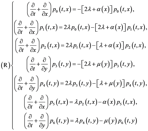
The system can be described by the following partial differential equations (see [4]).
with the boundary condition
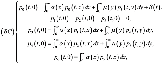
and the initial condition
 where
where 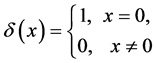
Here ;
;  gives the probability that at time t two units are operating, one unit is under standby, the repairman is in vacation, the system is good and the elapsed repair time lies in
 ;
;  represents the probability that at time
  two units are operating, one unit is waiting for repair, the repairman is in vacation, the system is good and the elapsed repair time lies in
 ;
;  represents the probability that at time
  two unit is operating, one unit is waiting for repair, the repairman is in vacation, the system is good and the elapsed repair time lies in
 ;
;  represents the probability that at time
  two units are operating, one unit being repaired, the system is good and the hours that the failed unit has been repaired lies in
 ;
; ![]() represents the probability that at time
represents the probability that at time ![]() one unit is operating, one unit being repaired, one unit is waiting for repair, the system is good and the hours that the failed unit has been repaired lies in
one unit is operating, one unit being repaired, one unit is waiting for repair, the system is good and the hours that the failed unit has been repaired lies in![]() ;
; ![]() represents the probability that at time
represents the probability that at time ![]() three units are waiting for repair, the repairman is in vacation, the system is down and the elapsed repair time lies in
three units are waiting for repair, the repairman is in vacation, the system is down and the elapsed repair time lies in![]() ;
; ![]() represents the probability that at time
represents the probability that at time ![]() one unit being repaired, two unit is waiting for repair, the system is down and the hours that the failed unit has been repaired lies in
one unit being repaired, two unit is waiting for repair, the system is down and the hours that the failed unit has been repaired lies in![]() ;
; ![]() are positive constants;
are positive constants; ![]() is the vacation rate function;
is the vacation rate function; ![]() is the repair rate function.
is the repair rate function.
Throughout the paper we require the following assumption for the vacation rate function ![]() and the repair rate function
and the repair rate function![]() .
.
General Assumption 1.1: The functions ![]() and
and ![]() are measurable and bounded such that
are measurable and bounded such that
![]()
To apply semigroup theory we use the same method in [5] to rewrite in this section the system![]() ,
, ![]() ,
,![]() as an abstract Cauchy problem ([6], Def.II.6.1) on the Banach space
as an abstract Cauchy problem ([6], Def.II.6.1) on the Banach space![]() , where
, where
![]()
and
![]()
![]() .
.
To define the system operator ![]() we introduce a “maximal operator”
we introduce a “maximal operator” ![]() on X given as
on X given as
![]() , where
, where ![]()
To model the boundary conditions (BC) we take the “boundary space” ![]() and then define “boundary operators”
and then define “boundary operators” ![]() and
and ![]() as follows.
as follows.
![]()
and
![]() ,
,
where![]() ,
, ![]()
If the system operator ![]() on
on ![]() is then defined as
is then defined as
![]() ,
,
Then the above equations ![]() and
and ![]() are equivalent to the abstract Cauchy problem
are equivalent to the abstract Cauchy problem
![]() (ACP)
(ACP)
By a direct computation we obtain the explicit form of the elements in ![]() as follows.
as follows.
Lemma 2.1: For![]() , we have
, we have
![]() (1)
(1)
![]()
![]()
![]()
![]()
![]()
![]()
![]()
We define the operator ![]() as
as
![]()
And then using ([8], Lemma 1.2), the domain ![]() of the maximal operator
of the maximal operator ![]() decomposes as
decomposes as
![]() .
.
Moreover, since is surjective,
![]()
is invertible for each![]() , see ([8], Lemma 1.2]. We denote its inverse by
, see ([8], Lemma 1.2]. We denote its inverse by
![]()
and call it “Dirichlet operator”.
We can give the form of ![]() as follows, see [5].
as follows, see [5].
Lemma 2.2: For each![]() , the operator
, the operator ![]() has the form
has the form
![]() ,
,
where
![]()
![]()
![]()
![]()
![]()
![]()
For![]() , the operator
, the operator ![]() can be represented by the
can be represented by the ![]() -matrix
-matrix
![]() ,
,
where
![]()
![]()
![]()
![]()
![]()
![]()
![]()
![]()
To prove the asymptotic stability of the dynamic solution of the system we apply the following result, which can be found in [9].
Lemma 2.3 (The characteristic equation): Let![]() , then
, then
(i)![]() .
.
(ii) If ![]() and there exists
and there exists ![]() such that
such that![]() , then
, then
![]() .
.
We obtained the following results in [5].
Theorem 3.4: The operator ![]() generates a positive contraction
generates a positive contraction ![]() -semigroup
-semigroup![]() .
.
Theorem 3.5: The associated abstract Cauchy problem ![]() is well-posed.
is well-posed.
Theorem 3.6: The system ![]() and
and ![]() has a unique positive dynamic solution
has a unique positive dynamic solution
![]() .
.
3. The Asymptotic Stability of the Dynamic Solution
In this section, we will investigate the asymptotic stability of the dynamic solution of the system. We show first the following lemmas:
Lemma 3.1: For the operator ![]() we have
we have![]() .
.
Proof: By a straightforward calculation we see that the matrix ![]() is column stochastic and thus
is column stochastic and thus![]() . Applying Lemma 2.3 (i), we immediately obtain
. Applying Lemma 2.3 (i), we immediately obtain![]() .
.
Using Lemma 2.3 (ii) we can show that 0 is the only spectral value of A on the imaginary axis.
Lemma 3.2: The spectrum ![]() of A satisfies
of A satisfies![]() .
.
Proof: If![]() ,then it is not difficult to derive that
,then it is not difficult to derive that![]() , thus the spectral radius fulfills
, thus the spectral radius fulfills![]() . This implies
. This implies![]() . By Lemma 2.3 (ii) we obtain that
. By Lemma 2.3 (ii) we obtain that ![]() for all
for all![]() ,
,![]() , i.e.,
, i.e., ![]()
We can express the resolvent of ![]() in terms of the resolvent of
in terms of the resolvent of![]() , the Dirichlet operator
, the Dirichlet operator ![]() and the boundary operator in the following way.
and the boundary operator in the following way.
Lemma 3.3: If![]() ,then
,then![]() .
.
Lemma 3.4: The semigroup ![]() generated by
generated by ![]() is irreducible.
is irreducible.
Proof: We can see as in ([9], Lemma 3.9) that ![]() transforms any positive vector
transforms any positive vector ![]() into a strictly positive vector. Using ([7], Def. C-III 3.1) this implies that the semigroup
into a strictly positive vector. Using ([7], Def. C-III 3.1) this implies that the semigroup ![]() generated by
generated by ![]() is irreducible.
is irreducible.
With this at hand one can then show the convergence of the semigroup to a one dimensional equilibrium point, see ([9], Th. 3.11).
Theorem 3.5: The space ![]() can be decomposed into the direct sum
can be decomposed into the direct sum
![]()
where ![]() is one-dimensional and spanned by a strictly positive eigenvector
is one-dimensional and spanned by a strictly positive eigenvector ![]() of
of![]() . In addition, the restriction
. In addition, the restriction ![]() is strongly stable.
is strongly stable.
Corollary 3.6: For all![]() , there exists
, there exists![]() , such that
, such that
![]()
where ![]()
Applying the above corollary, we now obtain our main result as follows.
Corollary 3.7: The dynamic solution of the system ![]() and
and ![]() converges strongly to the steady-state solution as time tends to infinity, that is,
converges strongly to the steady-state solution as time tends to infinity, that is,
![]()
where ![]() and
and ![]() as in Corollary 3.6.
as in Corollary 3.6.
Acknowledgements
This work was supported by the National Natural Science Foundation of China (No. 11361057).