Stability Analysis of a Delayed HIV/AIDS Epidemic Model with Treatment and Vertical Transmission ()
1. Introduction
Mathematical models play an important role in the study of the transmission dynamics of HIV/AIDS, and in some sense, delay models give better compatibility with reality, as they capture the dynamics from the time of infection to the infectiousness. Some HIV/AIDS models are introduced in [1] -[5] . In recent years, a few studies of vertical transmission have been conducted to describe the effects of various epidemiological and demographical factors [6] - [8] , and some models considered vertical transmission with time delay [9] [10] . Some specific HIV models with imperfect vaccine were introduced in [11] - [13] .
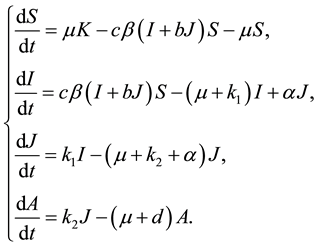
In [1] , L. Cai and X. Li studied local and global stability of the equilibria of a SIJA model with treatment:
 (1)
(1)
In model (1), it is assumed that some individuals with the symptomatic phases J can be transformed into asymptomatic individuals I after treatment and they get the result that when  the disease free equilibrium is globally asymptotically stable and if
  the endemic equilibrium is globally asymptotically stable.
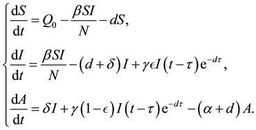
In [9] , Ram Naresh et al. considered the following SIA model with vertical transmission:
 (2)
(2)
Here, the authors assume that a fraction of newborns, who sustain treatment, join the infective class while others, who do not sustain treatment, join the AIDS class after getting sexual maturity. The infectives through vertical transmission at any time t are given by . The authors proved the local and global stability of disease free equilibrium and endemic equilibrium under some conditions. Inspired by these works, we consider an HIV/AIDS model with vertical transmission and with time delay.
The organization of the paper is as follows. In the next section we present the model with delay. Section 3 presents the basic properties of the model. In Section 4, we analyze local and global stability of equilibrium points. In the last section, we present a brief conclusion.
2. Mathematical Model
We propose an HIV/AIDS model which incorporates time delay during which a newly born infected child attains sexual maturity and becomes infectious. In this model, the sexually mature population is divided into four subclasses: the susceptibles (S), the asymptomatic infectives (I), the symptomatic infectives (J) and full-blown AIDS group (A). The number of total population is denoted by , for any time t. We assume that the susceptibles become HIV infected via sexual contacts with infectives. It is also assumed that all newborns are infected at birth
 . It is reasonable to assume that full-blown AIDS patients are sexually inactive and symptomatic stage patients feel uncomfortable (some may know they are AIDS) and the possibility of producing children is small, so can be taken negligible. We also assume that a fraction of infected newborns, who sustain treatment, joins the asymptomatic infective class while others, who do not sustain treatment, joins AIDS class after getting sexual maturity. The infectives through vertical transmission at any time t is given by
 , because those who are infected at time
  becomes infectoius (asymptomatic stage infectious) at time t, if they do not develop to AIDS patient by that time. The fraction of infectives which became AIDS patient during the period of getting sexual maturity, if they survive to the maturity, joins to the AIDS class. However, for the model to be biologically reasonable, it may be more realistic to assume that not all those infected will survive after
  time units, and this claim support the introduction of the survival term
 . Thus, in our model the term
  also represents the introduction of infectives through vertical transmission. If the birth rate of newborns
  equals to zero, then our model will back to the model (1).
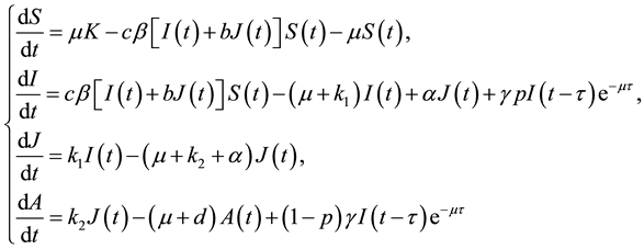
With the above considerations and assumptions, the spread of the disease is assumed to be governed by the following model:
 (3)
(3)
where  is the recruitment rate of the population,
  is the death rate. c is the average number of contacts of an individual per unit of time.
 ![]() and
and ![]() are the probability of disease transmission per contact by an infective in the first stage and in the second stage, respectively.
are the probability of disease transmission per contact by an infective in the first stage and in the second stage, respectively. ![]() and
and ![]() are transfer rate from the asymptomatic phase I to the symptomatic phase J and from the symptomatic phase to the AIDS cases, respectively.
are transfer rate from the asymptomatic phase I to the symptomatic phase J and from the symptomatic phase to the AIDS cases, respectively. ![]() is transformation rate from the symptomatic phase J to asymptomatic phase I. d is the disease-related death rate of the AIDS cases.
is transformation rate from the symptomatic phase J to asymptomatic phase I. d is the disease-related death rate of the AIDS cases. ![]() is the birth rate of infected newborns, p is the fraction of infected newborns joining the asymptomatic infective class after getting sexual maturity and remaining part
is the birth rate of infected newborns, p is the fraction of infected newborns joining the asymptomatic infective class after getting sexual maturity and remaining part ![]() of the infected newborns joins the AIDS class after getting sexual maturity
of the infected newborns joins the AIDS class after getting sexual maturity![]() . It is also assumed that all the parameters of the model are non-negative. Based on it’s biological meaning, we always assume that
. It is also assumed that all the parameters of the model are non-negative. Based on it’s biological meaning, we always assume that![]() .
.
3. Basic Properties
For model (2), let the initial condition be![]() ,
, ![]() ,
, ![]() ,
, ![]() for all
for all![]() , with
, with![]() . Then, it is clear that the solution
. Then, it is clear that the solution ![]() of the model (3) remain positive for all time
of the model (3) remain positive for all time![]() .
.
Let![]() , then
, then
![]()
which gives,
![]()
Define
![]()
This implies that if ![]() all solutions of model (3) starting in
all solutions of model (3) starting in ![]() are bounded and eventually enter the attracting set
are bounded and eventually enter the attracting set![]() .
.
It is reasonable to assume that the general death rate ![]() is greater than the birth rate of infected newborns
is greater than the birth rate of infected newborns![]() , that is
, that is![]() . In some models, death rate equal to birth rate. However, in this model,
. In some models, death rate equal to birth rate. However, in this model, ![]() is smaller than birth rate. Below we assume
is smaller than birth rate. Below we assume![]() .
.
Since the variable A of model (3) does not appear in the first three equation, in the subsequent analysis, we only consider the submodel:
![]() (4)
(4)
Model (4) always has a disease-free equilibrium![]() . Further we define the basic reproduction number
. Further we define the basic reproduction number ![]() as follows.
as follows.
![]()
By straightforward computation, when ![]() model (4) has the unique positive equilibrium
model (4) has the unique positive equilibrium![]() , where
, where
![]()
4. Stability Analysis
First we will study the local and global stability of disease free equilibrium![]() .
.
The variational matrix of model (4) is given by
![]()
Theorem 4.1. If![]() , the disease free equilibrium
, the disease free equilibrium ![]() is locally asymptotically stable.
is locally asymptotically stable.
Proof. The Jacobian matrix corresponding to model (4) about ![]() as follows,
as follows,
![]()
where![]() ,
,![]() .
.
The characteristic equation of this matrix is given by![]() , where I is the unit matrix.
, where I is the unit matrix.
![]() (5)
(5)
where
![]()
Clearly, one root of this equation is![]() . So we consider the following equation.
. So we consider the following equation.
![]() (6)
(6)
If![]() , the equation becomes
, the equation becomes
![]()
Since
![]()
when![]() , notice that
, notice that![]() ,
,![]() . Hence the roots of this equation have negative real part by the Hurwitz criterion.
. Hence the roots of this equation have negative real part by the Hurwitz criterion.
If![]() , we assume that
, we assume that ![]() is the root of characteristic Equation (6), then
is the root of characteristic Equation (6), then ![]() satisfies
satisfies
![]()
Separating the real and imaginary parts, we have
![]()
Eliminating ![]() by squaring and adding above the two equation, we get that
by squaring and adding above the two equation, we get that
![]()
Let![]() , then this equation becomes
, then this equation becomes
![]() (7)
(7)
Through simple computation, we can found that all the coefficients of this equation is positive, so Equation (7) have no solution, it implies that Equation (6) have not the root like![]() . Hence all roots of (6) have negative real part.
. Hence all roots of (6) have negative real part.
We are now in a position to investigate the global stability of the disease-free equilibrium![]() .
.
Theorem 4.2. If![]() , then the infection free equilibrium
, then the infection free equilibrium ![]() is globally asymptotically stable.
is globally asymptotically stable.
Proof. Consider the following Lyapunov functional.
![]()
Calculating the derivative of L along with the solution of model (4), we have
![]()
This implies that ![]() when
when![]() , the equality
, the equality ![]() holds if and only if
holds if and only if![]() , the maximal
, the maximal
invariant set of ![]() is the singleton
is the singleton![]() . Hence
. Hence ![]() is globally asymptotically stable by the LaSalle invariance principle [14] .
is globally asymptotically stable by the LaSalle invariance principle [14] .
Now, when ![]() we will study the local and global stability of
we will study the local and global stability of![]() .
.
Theorem 4.3. If![]() , the infected equilibrium
, the infected equilibrium ![]() is locally asymptotically stable.
is locally asymptotically stable.
Proof. For this purpose, we obtain the Jacobian matrix corresponding to model (4) about ![]() as follows,
as follows,
![]()
where![]() ,
, ![]() ,
,![]() .
.
The characteristic equation of this matrix is
![]() (8)
(8)
where
![]()
Notice that
![]()
Hence
![]()
when![]() , the characteristic Equation (8) yields
, the characteristic Equation (8) yields
![]()
where
![]()
Obviously, ![]() and
and![]() . This implies that when
. This implies that when ![]() and
and![]() ,
, ![]() is locally asymptotically stable by the Hurwitz criterion.
is locally asymptotically stable by the Hurwitz criterion.
Now we study the stability behavior of ![]() in the case
in the case![]() .
.
We assume that ![]() is the root of characteristic equation, then
is the root of characteristic equation, then ![]() satisfies
satisfies
![]()
Separating the real and imaginary parts, we have
![]() (9)
(9)
![]() (10)
(10)
Eliminating ![]() by squaring and adding (9) and (10), we get the equation determining for
by squaring and adding (9) and (10), we get the equation determining for ![]() as,
as,
![]()
where
![]()
Substituting ![]() in above Equation, we have
in above Equation, we have
![]() (11)
(11)
when![]() , through simple computation we can see that
, through simple computation we can see that![]() ,
, ![]() ,
, ![]() , in this circumstance (11) has not positive root. So all roots of (8) has negative real part.
, in this circumstance (11) has not positive root. So all roots of (8) has negative real part.
Next, we consider the global stability of ![]() when
when![]() .
.
Theorem 4.4. If![]() , then the infected equilibrium
, then the infected equilibrium ![]() is globally asymptotically stable.
is globally asymptotically stable.
Proof. Firstly, we define a function, ![]() ,
,![]() . Take the Lyapunov functional as follows.
. Take the Lyapunov functional as follows.
![]()
Next calculating the derivative of V along with the solution of model (4), we have
![]()
Since![]() , we have
, we have
![]()
Next,we consider the following variables substitutions by letting,
![]()
Then,
![]()
Further let
![]()
Then, through a straight computation, we have
![]()
Since the arithmetic mean is greater than or equal to the geometric mean and function g is a positive function, we have
![]()
Thus, ![]() in
in![]() . The equality
. The equality ![]() holds if and only if
holds if and only if![]() . That is,
. That is,![]() . The maximal invariant set of model (4) on the set
. The maximal invariant set of model (4) on the set ![]() is the singleton
is the singleton![]() . Thus, the endemic equilibrium
. Thus, the endemic equilibrium ![]() is globally asymptotically stable if
is globally asymptotically stable if ![]() by LaSalle Invariance Principle [14] .
by LaSalle Invariance Principle [14] .
5. Conclusion
In this paper, we have considered an HIV/AIDS model with treatment, vertical transmission and time delay. Under the assumption that asymptomatic infectives (J) have the symptoms of AIDS, AIDS patients (A) are isolated; hence their probability of producing children is small; and it is neglected. From the local stability of disease free equilibrium, we calculated the basic reproduction number![]() . Further we get the results that when
. Further we get the results that when ![]() the disease free equilibrium is globally asymptotic stable, and when
the disease free equilibrium is globally asymptotic stable, and when ![]() the endemic equilibrium is globally asymptotic stable.
the endemic equilibrium is globally asymptotic stable.
Acknowledgements
This work was supported by the National Natural Science Foundation of China (Grants nos. 11261056, 11261058 and 11271312).
NOTES
*Corresponding author.