1. Introduction
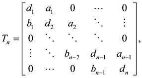
In many scientific and engineering applications, different special linear systems of equations arise. For such systems the coefficient matrix has special structure. Sparse matrices which contain a majority of zeros occur are often encountered. It is usually more efficient to solve these systems using tailor-made algorithms, much faster and with less storage than a full matrix. This can be achieved by taking advantage of the special structure of the coefficient matrix. Important examples are tridiagonal matrices. Tridiagonal systems of linear equations take the form:
 (1)
(1)
where
 (2)
(2)
 and
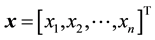
and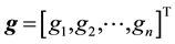 . The superscript T corresponds to the transpose operation. This type of matrices frequently appears in many applications, for example in parallel computing, telecommunication system analysis, solving differential equations using finite differences, heat conduction and fluid flow problems. A general
  tridiagonal matrix of the form (2) can be stored in
  memory locations, rather than
  memory locations for a full matrix, by using three vectors
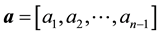 ,
,  , and
, and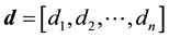 . This is always a good habit in computation in order to save memory space. To study tridiagonal matrices it is convenient to introduce a vector e defined by [1] [2] :
 (3)
(3)
where
 (4)
(4)
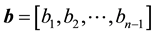
For some important results concerning tridiagonal matrix the reader may refer to [2] -[18] . The motivation of the current paper is to derive algorithms for solving bordered k-tridiagonal linear systems of the form:
 (5)
(5)
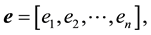
with
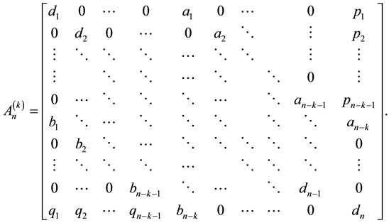 (6)
(6)
where ,
,  and
and![]() .
.
The linear systems (5) for![]() , frequently occur in engineering computation and analysis, e.g. in computation of electric power system and in solution of partial differential equations, as referred in [19] -[28] .
, frequently occur in engineering computation and analysis, e.g. in computation of electric power system and in solution of partial differential equations, as referred in [19] -[28] .
Throughout this paper, ![]() denotes the greatest integer less than or equal to x. Also, the word “simplify” means simplify the algebraic expression under consideration to its simplest rational form.
denotes the greatest integer less than or equal to x. Also, the word “simplify” means simplify the algebraic expression under consideration to its simplest rational form.
The organization of the paper is as follows: The main results are given in Section 2 and Section 3. Some illustrative examples are given in Section 4. A conclusion is given in Section 5.
2. Solving the System (5) via k-Tridiagonal Solvers
In this section, we are going to formulate a new symbolic algorithm, based on the Sherman-Morrison-Woodbury formula [29] , for solving bordered k-tridiagonal linear system of the form (5). By doing this, the solution of the system (5) reduces to solving three k-tridiagonal linear systems by using k-tridiagonal solvers such as these presented in [12] [30] .
Let us first note that the coefficient matrix, ![]() of the system (5) can be written as:
of the system (5) can be written as:
![]() (7)
(7)
where![]() , U and v are given by:
, U and v are given by:
![]() , (8)
, (8)
![]() (9)
(9)
and
![]() (10)
(10)
By applying the Sherman-Morrison-Woodbury formula to ![]() in (7), we get:
in (7), we get:
![]() (11)
(11)
and
![]() (12)
(12)
provided that the matrix ![]() in (8) is invertible.
in (8) is invertible.
By making use of (7)-(12), we see that the solution of the bordered k-tridiagonal system (5) reduces to solving three k-tridiagonal linear systems by using k-tridiagonal solvers. Consequently, we may formulate the following symbolic algorithm for solving the linear system (5).
Algorithm 2.1. An algorithm for solving bordered k-tridiagonal linear systems.
To solve bordered k-tridiagonal linear systems of the form (5), we may proceed as follows:
INPUT: The entries of the matrix ![]() in (8) and the vectors V, U and f.
in (8) and the vectors V, U and f.
OUTPUT: The solution vector ![]()
Step 1: Use the k-DETGTRI algorithm [12] to check the non-singularity of the matrix ![]() in (8).
in (8).
Step 2: If ![]() then Exiterror (“Failure”) end if.
then Exiterror (“Failure”) end if.
Step 3: Solve the three linear systems of k-tridiagonal type:
![]() ,
,![]() and
and![]()
by using, for example, the k-Thomas solver in [12] then construct![]() .
.
Step 4: Compute the ![]() matrix, H using
matrix, H using![]() .
.
If ![]() then Exiterror (“Failure”) end if.
then Exiterror (“Failure”) end if.
Step 5: Compute ![]() to get the solution vector x.
to get the solution vector x.
The computational cost of the algorithm is![]() . The Algorithm 2.1, will be referred to as DB-kTRI1 algorithm. Parallel computations of the three linear systems in Step 3 are available for heterogeneous environments.
. The Algorithm 2.1, will be referred to as DB-kTRI1 algorithm. Parallel computations of the three linear systems in Step 3 are available for heterogeneous environments.
It should be noted that the algorithm presented in [28] is a special case of the DB-kTRI1 algorithm when![]() .
.
3. Solving the System (5) Using the LU Factorization and Partition
In this section, we are going to consider the construction of a new algorithm for solving linear systems of equations of bordered k-tridiagonal type (5) by using partition. For this purpose it is convenient to introduce a vector![]() , whose first
, whose first ![]() components,
components, ![]() are given by:
are given by:
![]() (13)
(13)
where ![]() The last component,
The last component, ![]() of the vector c will be computed later on.
of the vector c will be computed later on.
Consider the Doolittle LU factorization [31] of the coefficient matrix ![]() in (6).
in (6).
![]() (14)
(14)
where![]() ,
, ![]() ,
, ![]() and
and ![]() is the
is the ![]() th leading principal submatrix of
th leading principal submatrix of![]() .
.
Equation (14) can be rewritten in the form:
![]() (15)
(15)
where
![]() (16)
(16)
![]() and
and![]() ,
,![]() .
.
From (15), we see that the following four matrix equations must be satisfied.
![]() (17)
(17)
![]() (18)
(18)
![]() (19)
(19)
and
![]() (20)
(20)
Two cases will be considered:
CASE(I):![]() :
:
In this case, solving (18) and (19) for h and v respectively, yields:
![]() (21)
(21)
![]() (22)
(22)
CASE(II):![]() :
:
In this case, solving (18) and (19) for h and v respectively, gives:
![]() (23)
(23)
![]() (24)
(24)
In both cases, we have from (20),
![]() (25)
(25)
At this stage, the determinant of the coefficient matrix in (6) can be computed using the following computational symbolic algorithm.
Algorithm 3.1. An algorithm for computing the determinant of bordered k-tridiagonal matrices.
To compute the determinant of a bordered k-tridiagonal matrix in (6), we may proceed as follows:
INPUT: Order of the matrix n, the value of k and the components,![]() .
.
OUTPUT: The determinant of the matrix ![]() in (6).
in (6).
Step 1: Compute![]() ,
, ![]() using (13).
using (13).
If ![]() for any
for any![]() , set
, set ![]() (t is just a symbolic name) and continue to compute
(t is just a symbolic name) and continue to compute
![]() , in its simplest rational forms, in terms of t using (13).
, in its simplest rational forms, in terms of t using (13).
Step 2: Compute ![]() using (25).
using (25).
Step 3: Simplify ![]() to obtain
to obtain![]() .
.
The Algorithm 3.1, will be referred to as DB-kDETGTRI algorithm.
Remarks:
1) The DETGTRI algorithm in [1] is a special case of DB-kDETGTRI algorithm when![]() ,
, ![]() and
and![]() .
.
2) The k-DETGTRI algorithm in [12] is a special case of DB-kDETGTRI algorithm when ![]()
![]() and
and![]() .
.
3) The PERTRI algorithm in [8] is a special case of DB-kDETGTRI algorithm when![]() ,
, ![]() and
and![]() ,
, ![]() , and
, and![]() .
.
4) The DETSGCM algorithm in [32] is a special case of DB-kDETGTRI algorithm when ![]()
![]()
![]()
![]() ,
, ![]()
![]() ,
, ![]()
![]() ,
, ![]() ,
, ![]() and
and![]() ,
, ![]() , and
, and![]() . (See also [33] ).
. (See also [33] ).
Now the linear system in (5), can be rewritten in partitioned form as:
![]() (26)
(26)
where![]() ,
, ![]() ,
, ![]() and
and![]() .
.
To solve the linear system (26) it is equivalent to solve the two standard linear systems:
![]() (27)
(27)
and
![]() (28)
(28)
where ![]() and
and![]() . The linear systems (27) and (28) can be solved directly by using forward and backward substitution respectively.
. The linear systems (27) and (28) can be solved directly by using forward and backward substitution respectively.
In conclusion, we may now formulate a second symbolic algorithm for solving the bordered k-tridiagonal linear system (5) as follows:
Algorithm 3.2. A symbolic algorithm for solving bordered k-tridiagonal linear systems using partition.
To solve a general bordered k-tridiagonal linear system of the form (5), we may proceed as follows:
INPUT: Order of the matrix n, the value of k and the components, ![]() and
and![]() .
.
OUTPUT: The determinant of the matrix ![]() in (6) and the solution vector
in (6) and the solution vector![]() .
.
Step 1: If ![]() then
then
For ![]() do
do
Set![]() , If
, If ![]() then
then ![]() End if
End if
![]() ,
,![]() ,
,![]() and
and![]() .
.
End do
For ![]() do
do
Compute and simplify:
![]() . If
. If![]() . then
. then ![]() End if
End if
![]()
![]()
![]()
End do.
For ![]() do
do
Compute and simplify:
![]() . If
. If ![]() then
then ![]() End if
End if
End do.
![]()
![]()
For ![]() do
do
Compute and simplify:
![]()
![]()
End do.
Else
For ![]() do
do
Set![]() , If
, If ![]() then
then ![]() End if
End if
![]()
End do
For ![]() do
do
Compute and simplify:
![]()
![]() If
If ![]() then
then ![]() End if
End if
End do.
For ![]() do
do
Compute and simplify:
![]()
![]()
End do.
![]()
![]()
For ![]() do
do
Compute and simplify:
![]()
![]()
End do.
For ![]() do
do
Compute and simplify:
![]()
![]()
End do.
End if
Step 2: Compute and simplify:
![]()
Step 3: Use the DB-kDETGTRI algorithm to check the non-singularity of the coefficient matrix of the system (5).
Step 4: If the determinant of the coefficient matrix in (5) equals zero, then Exiterror (“No solutions”) End if.
Step 5: Compute the solution vector ![]() using
using
For ![]() do
do
Compute and simplify:
![]()
End do.
![]()
![]()
Step 6: For ![]() do
do
Compute and simplify:
![]()
End do.
For ![]() do
do
Compute and simplify:
![]()
End do.
Step 7: Substitute ![]() in all expressions of the solution vector
in all expressions of the solution vector ![]()
Concerning the computational cost of Algorithm 3.2, we have: For ![]() the computational cost is
the computational cost is ![]() multiplications/divisions and
multiplications/divisions and ![]() additions/subtractions. The computational cost for the case
additions/subtractions. The computational cost for the case ![]() is
is ![]() multiplications/divisions and
multiplications/divisions and ![]() additions/subtractions. The Algorithm 2.3, will be referred to as DB-kTRI2 algorithm.
additions/subtractions. The Algorithm 2.3, will be referred to as DB-kTRI2 algorithm.
Remarks:
・ The DB-kTRI2 algorithm is a natural generalization of the algorithms in [30] and [34] .
・ The last component, ![]() of the vector a is also the (n-k)th component of the vector p.
of the vector a is also the (n-k)th component of the vector p.
・ The last component, ![]() of the vector b is also the (n-k)th component of the vector q.
of the vector b is also the (n-k)th component of the vector q.
A MAPLE procedure, based on the algorithm DB-kDETGTRI and DB-kTRI2, is available upon request from the authors.
4. Illustrative Examples
Example 4.1. Solve the bordered k-tridiagonal linear system
![]()
Solution: We have:![]() ,
, ![]() ,
, ![]() ,
, ![]() ,
, ![]() ,
, ![]() ,
, ![]() and
and![]() .
.
By applying the DB-kTRI1 algorithm, we get
・ ![]()
・ ![]() Thus
Thus ![]() is nonsingular, (Steps 1, 2).
is nonsingular, (Steps 1, 2).
・ ![]()
![]() (Step 3).
(Step 3).
・ ![]() (Step 4).
(Step 4).
・ The solution vector is ![]() (Step 5).
(Step 5).
Example 4.2. Solve the bordered k-tridiagonal linear system
![]()
Solution: We have:![]() ,
, ![]() ,
, ![]() ,
, ![]()
![]() ,
, ![]() ,
, ![]() and
and![]() .
.
By applying the DB-kTRI2 algorithm, we have
・ ![]()
・ ![]() . Hence
. Hence ![]() is nonsingular, (Steps 3, 4).
is nonsingular, (Steps 3, 4).
・ The solution vector is![]() , (Steps 5-7).
, (Steps 5-7).
Example 4.3. Solve the bordered k-tridiagonal linear system
![]()
Solution: We have:![]() ,
, ![]() ,
, ![]() ,
, ![]() ,
, ![]() ,
, ![]() ,
, ![]() and
and![]() .
.
By applying the DB-kTRI1 algorithm, we get
・ ![]()
・ ![]() Thus
Thus ![]() is nonsingular, (Steps 1, 2).
is nonsingular, (Steps 1, 2).
・ ![]()
![]() (Step 3).
(Step 3).
・ ![]() (Step 4).
(Step 4).
・ The solution vector is ![]() (Step 5).
(Step 5).
By applying the DB-kTRI2 algorithm, we have
・ ![]()
・ ![]() Hence
Hence ![]() is nonsingular, (Steps 3, 4).
is nonsingular, (Steps 3, 4).
・ The solution vector is ![]() (Steps 5-7).
(Steps 5-7).
5. Conclusion
In this paper we have derived two symbolic algorithms (DB-kTRI1 and DB-kTRI2) for solving bordered k- tridiagonal linear systems. The cost of each algorithm is![]() . Our algorithm does not require any simplifying assumptions. To the best of our knowledge, this is the first study to show how to solve bordered k-tridiagonal linear systems. Finally, three examples are given for the sake of illustration.
. Our algorithm does not require any simplifying assumptions. To the best of our knowledge, this is the first study to show how to solve bordered k-tridiagonal linear systems. Finally, three examples are given for the sake of illustration.
NOTES
*Corresponding author.