High Moments Jarque-Bera Tests for Arbitrary Distribution Functions ()
1. Introduction
In this paper, we are concerned with generalizations of Jarque-Bera’s (JB) [1] tests based on arbitrary first (4k) moments, k ≥ 2, rather than on the first eight ones as usual. (See [2] for a reminder of JB tests, page 69). We obtain general statistics that allow statistical tests for any distribution function G provided it has enough moments. For a reminder, the classical JB test belongs to the class of omnibus moment tests, i.e. those which assess simultaneously whether the skewness and kurtosis of the data are consistent with a Gaussian model. This test proves optimum asymptotic power and good finite sample properties (see [1] ). A detailed description of that test and related indepth analyses can be found in Bowman and Shenton, D’Agosto, D’Agostino et al., etc. (see [3] -[5] and [6] ).
Let  be a sequence of independent and identically distributed random variables (r.v.’s) defined on the same probability space
 . For each
 , the skewness and kurtosis coefficients related to the sample
  are defined by.
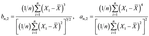 (1)
(1)
These statistics are designed to estimate the theoretical skewness and kurtosis given by  and
and 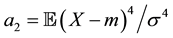 where
where  and
and  respectively denote the mean and the variance of X that is supposed to be nondegenerated. Here and in all the sequel,
  stands for the mathematical expectation with respect to the probability
 . Now, under the hypothesis:
H0: X follows a Gaussian normal law, we have  and
and  and the JB statistic
 (2)
(2)
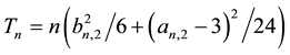
has an asymptotic chi-square distribution with two degrees of freedom under the null hypothesis of normality. Jarque-Bera’s test consists in rejecting H0 when Tn is far from zero. We will find below that the constants 6 and 24 used in (2), actually, are closely related to the first four even moments of a  random variable which are 1, 3, 15 and 105 and a more convenient form of (2) is
Our objective here is to generalize JB’s test to a general df G by considering high moments![]() ,
, ![]() , with
, with![]() , instead of the first eight moments only. We base our methods on the remark that for a random variable
, instead of the first eight moments only. We base our methods on the remark that for a random variable![]() , one has
, one has
![]() . (H1)
. (H1)
Actually, JB’s test only checks the third and fourth moments of X while the coefficients of the JB statistic (2) uses the first eight moments of X. Our guess is that we would have better tests if we are able to simultaneously check all the first (2k) moments for some k ≥ 2. To this purpose, we consider the following statistics, that is the normalized centered empirical moments (NCEM),
![]() (3)
(3)
where
![]()
are the ![]() non-centered and the centered empirical moments. By the classical law of large numbers, the statistics in (3) are, for each fixed p, asymptotic estimators of
non-centered and the centered empirical moments. By the classical law of large numbers, the statistics in (3) are, for each fixed p, asymptotic estimators of
![]() , (4)
, (4)
whenever the (4p)th moment exists. Finally we consider C1-class functions ![]() et
et ![]() and denote
and denote ![]() and
and![]() .
.
Our general test is based on the following statistics, for k ≥ 2,
![]() (5)
(5)
which almost-surely ![]() tends to
tends to
![]() , (6)
, (6)
as![]() . For an independent and identically distributed sequence
. For an independent and identically distributed sequence ![]() of r.v.’s associated with a distribution function G having a finite 2k-moment, we will have by Theorem 1 below that
of r.v.’s associated with a distribution function G having a finite 2k-moment, we will have by Theorem 1 below that
![]()
From such a general result, we are able to derive a normality test by using it with![]() ,
, ![]() for
for![]() , and rejects normality for a large value of
, and rejects normality for a large value of![]() .
.
We are going to establish a general asymptotic normality of ![]() for any df’s G with 4k finite moments. These results provide themselves efficient tests for an arbitrary d.f. Next, we will derive chi-square tests that generalize JB’s test for higher moments and for arbitrary df’s too.
for any df’s G with 4k finite moments. These results provide themselves efficient tests for an arbitrary d.f. Next, we will derive chi-square tests that generalize JB’s test for higher moments and for arbitrary df’s too.
Our results will show that these tests based on the 2k moments, need, in fact, the eight 4k moments for computing the variance. This unveils that the classical JB’s test is not based only on the kurtosis and the skewness but also on the sixth and the eighth moments. To describe the complete form of the Jarque-Bera method, put
![]()
The JB’s test for a ![]() r.v. will be showed to derive from the following general law
r.v. will be showed to derive from the following general law
![]() . (7)
. (7)
with the particular coefficients![]() ,
, ![]() and
and![]() . This may be a new explanation of the powerfulness of the JB classical tests since a successful test of normality means that the sample is from a df having same first eight moments as the
. This may be a new explanation of the powerfulness of the JB classical tests since a successful test of normality means that the sample is from a df having same first eight moments as the ![]() r.v., and this is very highly improbable for a non normal r.v..
r.v., and this is very highly improbable for a non normal r.v..
As an illustration of what proceeds, consider a distribution following a double-gamma distribution
![]() of density probability
of density probability ![]() with
with![]() . This rv is
. This rv is
centered and has a kurtosis coefficient equal to 3. It is rejected from normality by the JB test. If only the skewned and kurtosis do matter, it would not be the case. Actually, the rejection comes from the parameters ![]() and
and ![]() that are very different from a standard normal distribution to this specific distribution.
that are very different from a standard normal distribution to this specific distribution.
The rest of the paper is organized as follows. In Subsection 2.1 of Section 2, we begin to give a concise of reminder the modern theory of functional empirical processes that is the main theoretical tool we use for finding the asymptotic law of (5). Next in Subsection 2.2, we establish general results of the consistency of (5) and its asymptotic law, consider particular cases in Subsection 2.3, propose chi-square universal tests in Subsection 2.4 and finally state the proofs in Subsection 2.5. We end the paper by Section 3 where simulation results concerning the normal and double-exponential models are given.
We here express that in all the sequel the limits are meant as ![]() and this will not be written again unless it is necessary.
and this will not be written again unless it is necessary.
2. Results and Proofs
2.1. A Reminder of Functional Empirical Process
Since the empirical functional process is our key tool here, we are going to make a brief reminder on this process associated with![]() , and defined for each
, and defined for each ![]() by
by
![]()
where f is a real measurable function defined on ![]() such that
such that
![]() , (8)
, (8)
and
![]() (9)
(9)
It is known (see van der Vaart [7] , pages 81-93) that ![]() converges to a functional Gaussian process
converges to a functional Gaussian process ![]() with covariance function
with covariance function
![]() (10)
(10)
at least in finite distributions. ![]() is linear, that is, for f and g satisfying (9) and for
is linear, that is, for f and g satisfying (9) and for![]() , we have
, we have
![]() .
.
This linearity will be useful for our proofs. We are now in position to state our main results.
2.2. Statements of Results
First introduce this notation for![]() ,
, ![]() , and
, and![]() . Let fi and gi,
. Let fi and gi, ![]() be C1-functions with values in
be C1-functions with values in![]() . Put
. Put ![]() and
and ![]() and
and![]() ,
, ![]() ,
,
![]() (11)
(11)
![]() (12)
(12)
![]() (13)
(13)
and
![]() (14)
(14)
Here are our main results.
Theorem 1 Let![]() , for
, for![]() . Then
. Then
![]() ,
,
where
![]() .
.
Corollary 1 (Normality test). Let X be a ![]() r.v. and let, for all
r.v. and let, for all ![]()
![]() ,
,
Then
![]() ,
,
where
![]() ,
,
and
![]() .
.
2.3. Particular Cases and Consequences
2.3.1. A General Test
Let G be an arbitrary df with a 4kth finite moment for k ≥ 2, this is![]() . We want to check whether a sample
. We want to check whether a sample ![]() is from G. We then select C1-functions fi and gi,
is from G. We then select C1-functions fi and gi, ![]() and compute the observed
and compute the observed
value ![]() of
of ![]() and report the p-value of the test, that is
and report the p-value of the test, that is
![]() where s2 is either the exact variance
where s2 is either the exact variance ![]() or its plug-in estimator
or its plug-in estimator
![]()
Our guess is that using a greater value of k makes the test more powerful since the equality in distribution of univariate r.v.’s means equality of all moments when they exist (see page 213 in [8] ). For k = 2, this result depends on the first eight moments. Then to find another df G1 for which the p-value exceeds 5% would suggest it has the same eight moments as G, which is highly improbable. Simulation studies in Section 0 support our findings. Remark that we have as many choices as possible for the functions the ![]() and
and![]() .
.
Unfortunately, in the simulation studies reported below, we noticed that the plug-in estimator ![]() may hugely over estimate the exact variance and leads to accepting any data to follow that model, or significantly underestimate it and leads to reject data from the model itself. This is why we only use the exact variance here.
may hugely over estimate the exact variance and leads to accepting any data to follow that model, or significantly underestimate it and leads to reject data from the model itself. This is why we only use the exact variance here.
Now let us show how to derive chi-square tests from Theorem 1.
2.3.2. Generalized JB Test and Tests for Symmetrical df’s
Suppose that X is a symmetrical distribution. We have from Theorem 1 that
![]() (15)
(15)
Since X is symmetrical, that is ![]() for
for![]() , we may without loss of generality suppose that
, we may without loss of generality suppose that ![]() since replacing X by
since replacing X by ![]() does affect neither the
does affect neither the ![]() nor the
nor the![]() . Then we have from (11) and (12) that
. Then we have from (11) and (12) that
![]()
and
![]()
By reminding that ![]() for
for ![]() and
and![]() , we observe that the product
, we observe that the product ![]() only includes functions
only includes functions ![]() with odd
with odd ![]() and then
and then![]() . Thus
. Thus
![]()
where![]() ,
, ![]() and
and![]() . We get
. We get
Corollary 2 Let ![]() for
for ![]() and G be a symmetrical df. We have
and G be a symmetrical df. We have
![]() . (16)
. (16)
For a standard normal random variable, we get ![]() and
and ![]() and the normality JB’s test becomes a particular case of (16), which is a general chi-square test for an arbitrary df with 2p-finite moments.
and the normality JB’s test becomes a particular case of (16), which is a general chi-square test for an arbitrary df with 2p-finite moments.
Corollary 3 Let G be a Gaussian df. Then
![]() .
.
We see that we obtain an infinite number of tests for the normality. For example, for![]() , we have,
, we have,
![]() , etc.
, etc.
2.4. A General Chi-Square Test
Consider (15) and put ![]() and suppose that
and suppose that![]() . We have
. We have
Corollary 4 Let ![]() and
and ![]() for
for![]() . Then
. Then
![]()
converges in law to a ![]() r.v..
r.v..
It is now time to prove Theorem 1 before considering the simulation studies.
2.5. Proofs
Since G has at least first 4k moments finite, we are entitled to use the finite-distribution convergence of the empirical function process ![]() as below. Let us begin to give the asymptotic law of
as below. Let us begin to give the asymptotic law of![]() . By denoting
. By denoting![]() , we have
, we have
![]()
where ![]() is defined in (11) and where we used that the linearity of the empirical functional process. By observing that
is defined in (11) and where we used that the linearity of the empirical functional process. By observing that![]() , we finally obtain
, we finally obtain
![]() . (17)
. (17)
Now the law of ![]() is given by
is given by
![]()
By the delta-method, we have
![]()
and then
![]()
and next, by noticing from 17 that ![]() for all
for all![]() ,
,
![]() ,
,
![]() ,
,
where ![]() is given in (12). By the very same methods, we have
is given in (12). By the very same methods, we have
![]() ,
,
![]() is stated in (13). The delta-method also yields
is stated in (13). The delta-method also yields
![]()
This completes the proof of the theorem. The proof of the corollary is a simple consequence of the theorem.
3. Simulation and Applications
3.1. Scope the Study
We want to focus on illustrating how performs the general test for usual laws such as Normal and Double Gamma ones. It is clear that the generality of our results that are applicable to arbitrary d.f.’s with some finite kth-moment ![]() deserves extended simulation studies for different classes of df’s. We particularly have to pay attention to the choice of k and of the functions fi and gi, depending on the specific model we want to test.
deserves extended simulation studies for different classes of df’s. We particularly have to pay attention to the choice of k and of the functions fi and gi, depending on the specific model we want to test.
In this paper, we want to set a general and workable method to simulate and test two symmetrical models. The normal and the double-exponential one with density![]() . We expect to find a test that accepts normality for normal data and rejects double-exponential data and to confirm this by the Jarque-Berra test, and to have another test that exactly does the contrary.
. We expect to find a test that accepts normality for normal data and rejects double-exponential data and to confirm this by the Jarque-Berra test, and to have another test that exactly does the contrary.
Once these results are achieved, we would be in position to handle a larger scale simulation research following the outlined method. Specially, fitting financial data to the generalized hyperbolic model is one the most interesting applications of our results.
3.2. The Frame
We first choose all the functions fi equal to f0 and all the functions gi equal to g0. We fix k = 3, that is we work with the first twelve moments. As a general method, we consider two df’s G1 and G2. We fix one of them say G1 and compute ![]() and the variance
and the variance ![]() from the exact distribution function G1. We generate samples of size n from one the df’s (either G1 or G2) and compute
from the exact distribution function G1. We generate samples of size n from one the df’s (either G1 or G2) and compute![]() . We repeat this B times
. We repeat this B times
and report the mean value t* of the replicated values of ![]() and report the
and report the
p-value![]() . The simulation outcomes will be considered as conclusive if p is high for samples from G1 and low for samples from G2. The results are compared with those given by the Kolmogorov- Smirnov test (KST) and when the data are Gaussian, they are compared with the outcomes from JB’s classical test.
. The simulation outcomes will be considered as conclusive if p is high for samples from G1 and low for samples from G2. The results are compared with those given by the Kolmogorov- Smirnov test (KST) and when the data are Gaussian, they are compared with the outcomes from JB’s classical test.
3.3. The Results
We consider the following cases: G1 is a Gaussian r.v![]() ; G2 is double-exponential law
; G2 is double-exponential law ![]() with density probability
with density probability ![]() and G3 is a double-gamma law
and G3 is a double-gamma law ![]() with probability den-
with probability den-
sity![]() .
.
Normal Model ![]()
The choice ![]() is natural since the Jarque-Berra test may be derived for our result for these functions and for
is natural since the Jarque-Berra test may be derived for our result for these functions and for![]() . The model is determined by these following parameters:
. The model is determined by these following parameters:
We recall that the variance of our statistic depends on the first 4k moments.
Simulation study.
Testing the model with ![]() data gives the following outcomes for
data gives the following outcomes for ![]()
and for n = 100,
and for n = 1000,
where JB is the classical Jarque-Berra statistic, pJB is the p-value of the JB test, KS is the Kolmogorov-smirnov statistic and pKS is the related p-value. Our model accepts the normality and this is confirmed by JB’s test and by the Klmogorov-Smirnov test (KST). The simulation results are very stable and constantly suggest acceptance.
Testing the double-exponential versus the normal model.
Recall that the values ![]() for
for ![]() are
are![]() ,
, ![]() ,
, ![]() ,
,![]() . Comparing these values with those of a normal model, it is natural to think that the test will fail since only the bp coincide and the test is only based on the moments. Indeed, using data from
. Comparing these values with those of a normal model, it is natural to think that the test will fail since only the bp coincide and the test is only based on the moments. Indeed, using data from ![]() gives for n = 11
gives for n = 11
and for n = 22
Our test rejects the ![]() model for n = 11 and JB’s test rejects it only for
model for n = 11 and JB’s test rejects it only for![]() . We see here the advantage brought by the value k = 3 in our statistic. The KST has problems in rejecting the false
. We see here the advantage brought by the value k = 3 in our statistic. The KST has problems in rejecting the false ![]() even for n = 1000 that of Jarque-Berra.
even for n = 1000 that of Jarque-Berra.
Testing the double-gamma versus the normal model.
Let use ![]() data with
data with ![]() and
and![]() . We have the outcomes for
. We have the outcomes for ![]()
and for n = 22
We have similar results. Ou test rejects the ![]() model for n = 12 and JB’s test rejects it only for n ≥ 18. We see here the advantage brought by the value k = 3 in our statistic. Although the first four moments of a
model for n = 12 and JB’s test rejects it only for n ≥ 18. We see here the advantage brought by the value k = 3 in our statistic. Although the first four moments of a ![]() are 0, 1, 0 and 3, that is, the same of those of standard normal rv, this model is rejected. We already pointed out that the coefficients 4 and 6 are in fact based on the first eight moments and the discrepancy of moments higher than 4 results in the rejection.
are 0, 1, 0 and 3, that is, the same of those of standard normal rv, this model is rejected. We already pointed out that the coefficients 4 and 6 are in fact based on the first eight moments and the discrepancy of moments higher than 4 results in the rejection.
Analysing the tables above, we conclude that our test performs better the JB’s test against a double-gamma df with same skewness and kurtosis than a normal df for small sample sizes around ten and this is real advantage for small data sizes. Even for k = 2, our test is performant for the small values n = 11 and n = 12.
Double-exponential model![]() .
.
We point out that the statistic ![]() does not depend on the
does not depend on the![]() . Then we only consider
. Then we only consider ![]() in the following. We always use
in the following. We always use![]() . The model is determined by the following values.
. The model is determined by the following values.
Here, we do not have the Jarque-Berra test to confirm the results.
Simulation. Testing the model with ![]() data gives the following outcomes, for n = 800.
data gives the following outcomes, for n = 800.
The simulation results are very stable and constantly suggest acceptance.
Testing normal data. Using normal data gives
The ![]() model is rejected. We noticed that the rejection of normal data is automatically obtained for large sizes here, when n is greater than 900. For n between 500 and 900, rejection is frequent but acceptance occurs now and then. Whe also noticed that the variance of
model is rejected. We noticed that the rejection of normal data is automatically obtained for large sizes here, when n is greater than 900. For n between 500 and 900, rejection is frequent but acceptance occurs now and then. Whe also noticed that the variance of ![]() are high and do not allow to reject normal data for small sizes. This leads us to consider other functions. Now consider the classes of functions
are high and do not allow to reject normal data for small sizes. This leads us to consider other functions. Now consider the classes of functions
![]() .
.
We obtain good results for ![]() with
with ![]() and
and![]() . In this case, the exact value of the statistic is 11.600. The double-exponential
. In this case, the exact value of the statistic is 11.600. The double-exponential ![]() model is confirmed according to the following table
model is confirmed according to the following table
while the normal model is rejected as illustrated below:
It is important to mention here that the KST is very powerful is rejecting the normal model with double-ex- ponential and double-gamma data with extremely low p-value’s.
3.4. Conclusion and Perspectives
We propose a general test for an arbitrary model. The methods are based on functional empirical processes theory that readily provides asymptotic laws from which statistical tests are derived. They depend on an integer k such that the pertaining df has 4k first finite moments. We get two kinds of tests. A general one based on functions fi and gi, ![]() , with an asymptotic normal law. We derive from these results chi-square tests that are valid for general df’s and that includes the Jarque-Berra test of normality. Both tests use arbitrary moments. We only undergo simulation studies for the first kind of test. Our simulation studies show high performance for nor- mality against other symmetrical laws such as double-exponential or double-gamma ones. For suitable choices of fi, gi, and k, the test performs well for small samples (n = 20) both for accepting the normal model and rejecting other models. We also show that for suitable choice of fi and gi, the test for the double-exponential model is also successful, but for sizes greater that n = 150. In upcoming papers, we will focus on detailed results on specific models and try to found out, for each case, suitable value of the parameters of the tests ensuring good performances for small data. A paper is also to be devoted to simulation studies for the khi-square tests and their applications to financial data.
, with an asymptotic normal law. We derive from these results chi-square tests that are valid for general df’s and that includes the Jarque-Berra test of normality. Both tests use arbitrary moments. We only undergo simulation studies for the first kind of test. Our simulation studies show high performance for nor- mality against other symmetrical laws such as double-exponential or double-gamma ones. For suitable choices of fi, gi, and k, the test performs well for small samples (n = 20) both for accepting the normal model and rejecting other models. We also show that for suitable choice of fi and gi, the test for the double-exponential model is also successful, but for sizes greater that n = 150. In upcoming papers, we will focus on detailed results on specific models and try to found out, for each case, suitable value of the parameters of the tests ensuring good performances for small data. A paper is also to be devoted to simulation studies for the khi-square tests and their applications to financial data.