Necessary Conditions for the Application of Moving Average Process of Order Three ()
1. Introduction
Moving average processes (models) constitute a special class of linear time series models. A moving average process of order  (
( process) is of the form:
 (1.1)
(1.1)
where  are real constants and
 ,
,  is a sequence of independent and identically distributed random variables with zero mean and constant variance. These processes have been widely used to model time series data from many fields [1] -[3] . The model in (1.1) is always stationary. Hence, a required condition for the use of the moving average process is that it is invertible. Let
 , then the model in (1.1) is invertible if the roots of the characteristic equation
 (1.2)
(1.2)
lie outside the unit circle. The invertibility conditions of the first order and second order moving average models have been derived [4] [5] .
Ref. [6] used a moving average process of order three (MA (3) process) in his simulation study. Though, higher order moving average processes have been used to model time series data, not much has been said about the properties of their autocorrelation functions. This study focuses on the invertibility condition of an MA (3) process. Consideration is also given to the properties of its autocorrelation coefficients of an invertible moving average process of order three.
2. Consequence of Invertibility Condition on the Parameters of an MA (3) Process
For , the following moving average process of order 3 is obtained from (1.1):
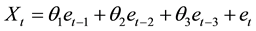 (2.1)
(2.1)
The characteristic equation corresponding to (2.1) is given by
 (2.2)
(2.2)
Dividing (2.2) by  yields
 (2.3)
(2.3)
It is important to know that (2.2) is a cubic equation. Detailed information on how to solve cubic equations can be found in [7] [8] among others. It has been a common tradition to consider the nature of the roots of a characteristic equation while determining the invertibility condition of a time series model [9] . As a cubic equation, (2.2) may have three distinct real roots, one real root and two complex roots, two real equal roots or three real equal roots. The nature of the roots of (2.2) is determined with the help of the discriminant [8]
![]() (2.4)
(2.4)
where
![]() (2.5)
(2.5)
and
![]() (2.6)
(2.6)
If![]() , (2.2) has the following distinct roots [7]
, (2.2) has the following distinct roots [7]
![]() , (2.7)
, (2.7)
![]() , (2.8)
, (2.8)
and
![]() . (2.9)
. (2.9)
where ![]() is measured in radians and
is measured in radians and![]() .
.
When![]() , (2.2) has only real root given by [1] as
, (2.2) has only real root given by [1] as
![]() (2.10)
(2.10)
The other roots are [8]
![]() (2.11)
(2.11)
If![]() ,
, ![]() and
and![]() , then
, then ![]() and (2.2) has two equal roots. The roots of (2.2) in this case, are the same as (2.7), (2.8) and (2.9). For
and (2.2) has two equal roots. The roots of (2.2) in this case, are the same as (2.7), (2.8) and (2.9). For ![]() and
and![]() , (2.2) has three real equal roots. Each of these roots is given by [8] as
, (2.2) has three real equal roots. Each of these roots is given by [8] as
![]() (2.12)
(2.12)
For (2.1) to be invertible, the roots of (2.2) are all expected to lie outside the unit circle and![]() . In the following theorem, the invertibility conditions of an MA (3) process are given subject to the condition that the corresponding characteristic equation has three real equal roots.
. In the following theorem, the invertibility conditions of an MA (3) process are given subject to the condition that the corresponding characteristic equation has three real equal roots.
Theorem 1. If the characteristic equation ![]() has three real equal roots, then the moving average process of order three
has three real equal roots, then the moving average process of order three ![]() is invertible if
is invertible if
![]() ,
,![]() and
and![]() .
.
Proof
For invertibility, we expect each of the three real equal roots to lie outside the unit circle. Thus,
![]() or
or ![]()
Solving the inequality![]() , we obtain
, we obtain
![]()
For![]() , we have
, we have
![]()
Since each of the roots lie outside the unit circle, the absolute value of their product must therefore be greater than one. Hence,
![]()
This completes the proof.
The invertibility region of a moving average of order three with equal roots of the characteristic Equation (2.2) is enclosed by triangle OAB in Figure 1.
![]()
Figure 1. Invertibility region of an MA (3) process when the characteristic equation has three real equal roots.
3. Identification of Moving Average Process
Model identification is a crucial aspect of time series analysis. A common practice is to examine the structures of the autocorrelation function (ACF) and partial autocorrelation function (PACF) of a given time series. In this regard, a time series is said to follow a moving average process of order ![]() if its associated autocorrelation function cut off after lag
if its associated autocorrelation function cut off after lag ![]() and the corresponding partial autocorrelation function decays exponentially [10] . Authors using this method, believe that each process has unique ACF representation. However, the existence of similar autocorrelation structures between moving average process and pure diagonal bilinear time series process of the same order makes it difficult to identify a moving average process based on the pattern of its ACF. Furthermore, a careful look at the autocorrelation function of the square of a time series can help one determine if the series follows a moving average process. If the series can be generated by a moving average process, then its square follows a moving average process of the same order [11] [12] . The conditions under which we use the autocorrelation function to distinguish among processes behaving like moving average processes of order one and two have been determined by [13] [14] respectively. These conditions are all defined in terms of the extreme values of autocorrelation coefficients of the processes.
and the corresponding partial autocorrelation function decays exponentially [10] . Authors using this method, believe that each process has unique ACF representation. However, the existence of similar autocorrelation structures between moving average process and pure diagonal bilinear time series process of the same order makes it difficult to identify a moving average process based on the pattern of its ACF. Furthermore, a careful look at the autocorrelation function of the square of a time series can help one determine if the series follows a moving average process. If the series can be generated by a moving average process, then its square follows a moving average process of the same order [11] [12] . The conditions under which we use the autocorrelation function to distinguish among processes behaving like moving average processes of order one and two have been determined by [13] [14] respectively. These conditions are all defined in terms of the extreme values of autocorrelation coefficients of the processes.
4. Intervals for Autocorrelation Coefficients of a Moving Average Process of Order Three
As stated in Section 3, knowledge of the extreme values of the autocorrelation coefficient of a moving average process of a particular order can enable us ensure proper identification of the process. It has been observed that for a moving average process of order one, ![]() [15] while for a moving average process of order
[15] while for a moving average process of order
two ![]() and
and ![]() [5] . In order to generalize about the range of values of
[5] . In order to generalize about the range of values of ![]() for a
for a
moving average process of order![]() , it is worthwhile to determine the range values of
, it is worthwhile to determine the range values of ![]() for a moving average process of order three. The model in (2.1) has the following autocorrelation function [10] :
for a moving average process of order three. The model in (2.1) has the following autocorrelation function [10] :
![]() (4.1)
(4.1)
We can deduce from (4.1) that the autocorrelation function at lag one of the MA (3) process is
![]() (4.2)
(4.2)
Using the Scientific Note Book, the minimum and maximum values of ![]() are found to be
are found to be ![]() and
and ![]() respectively. For the autocorrelation function at lag two, we have
respectively. For the autocorrelation function at lag two, we have
![]() (4.3)
(4.3)
The extreme values of ![]() are equally obtained with the help of the Scientific Note Book. To this effect,
are equally obtained with the help of the Scientific Note Book. To this effect, ![]() has a minimum value of −0.5 and a maximum value of 0.5.
has a minimum value of −0.5 and a maximum value of 0.5.
From (4.1), we obtain
![]() (4.4)
(4.4)
Based on the result obtained from the Scientific Notebook, ![]() has a minimum value of −0.5 and a maximum value of 0.5. However, the intervals for
has a minimum value of −0.5 and a maximum value of 0.5. However, the intervals for ![]() can easily be obtained analytically and this result is generalized in Theorem 2 for
can easily be obtained analytically and this result is generalized in Theorem 2 for ![]() of the MA
of the MA ![]() process.
process.
The partial derivatives of ![]() with respect to
with respect to![]() ,
, ![]() and
and ![]() are
are
![]() (4.5)
(4.5)
![]() (4.6)
(4.6)
![]() (4.7)
(4.7)
The critical points of ![]() occurs when
occurs when![]() ,
,![]() . Equating each of the partial derivatives in (4.5),
. Equating each of the partial derivatives in (4.5),
(4.6) and (4.7) to zero, we obtain
![]() (4.8)
(4.8)
![]() (4.9)
(4.9)
![]() (4.10)
(4.10)
From (4.10), we have
![]() (4.11)
(4.11)
Using (4.8), we obtain
![]() (4.12)
(4.12)
or
![]() (4.13)
(4.13)
Substituting ![]() into (4.11) yields
into (4.11) yields
![]() (4.14)
(4.14)
For![]() , (4.9) becomes
, (4.9) becomes
![]()
![]()
![]() (4.15)
(4.15)
If we also substitute ![]() into (4.9), we obtain
into (4.9), we obtain
![]() (4.16)
(4.16)
When we substitute ![]() and
and ![]() into (4.11), we have
into (4.11), we have![]() . It is also clear that if
. It is also clear that if ![]() and
and![]() , then
, then![]() . Similar result is obtained when
. Similar result is obtained when ![]() and
and![]() .
.
Hence, the critical points of ![]() are
are![]() ,
, ![]() ,
, ![]() and
and![]() .
.
The minimum and maximum values of a function occur at it critical points. To determine which of the critical points is a local minimum, local maximum or a saddle point, we shall apply the second derivative test. The second derivative test for critical points of a function of three variables ![]() focuses on the Hessian matrix:
focuses on the Hessian matrix:
![]() (4.17)
(4.17)
where
![]() (4.18)
(4.18)
![]() (4.19)
(4.19)
![]() (4.20)
(4.20)
![]() (4.21)
(4.21)
![]() (4.22)
(4.22)
![]() (4.23)
(4.23)
Let ![]() be a critical point of
be a critical point of![]() . Then
. Then ![]() is called a local minimum point if at
is called a local minimum point if at
![]() ,
, ![]() ,
, ![]() and
and ![]() [16] . If
[16] . If![]() ,
, ![]() and
and ![]() at
at![]() ,
,
then ![]() represents a local maximum.
represents a local maximum.
A critical point that is neither a local minimum nor a local maximum is called a saddle point.
Though ![]() has four critical points, it is not defined at
has four critical points, it is not defined at ![]() and
and![]() . We then focus on the classification of the two remaining critical points.
. We then focus on the classification of the two remaining critical points.
At ![]()
![]()
Hence, ![]() ,
, ![]() and
and![]() .
.
Therefore, ![]() is a local minimum. The value of
is a local minimum. The value of ![]() at this point is
at this point is![]() .
.
For the critical points![]() , we have
, we have
![]()
Consequently,
![]()
![]()
and
![]()
We therefore conclude that ![]() is a local maximum. The maximum value of
is a local maximum. The maximum value of ![]() obtained at
obtained at ![]() is 0.5.
is 0.5.
We can deduce from the result in this section and other previous works that for MA (1) process![]() , while for MA (2) process and MA (3) process
, while for MA (2) process and MA (3) process ![]() and
and ![]() respectively.
respectively.
In what follows, we establish the bounds for![]() , where
, where ![]() is order of the moving average process.
is order of the moving average process.
Theorem 2.
Let ![]() be an MA
be an MA ![]() process. Then,
process. Then,![]() .
.
Proof
It is easily seen that for the MA ![]() process,
process,
![]()
Partial derivatives of ![]() with respect to
with respect to ![]() are as follows
are as follows
![]()
Equating each of the partial derivatives to zero yields
![]() (4.24)
(4.24)
From (4.24), we obtain
![]() (4.25)
(4.25)
Since ![]() for an MA
for an MA ![]() process, it is obvious that the
process, it is obvious that the ![]() equations preceding (4.24) are only satisfied if
equations preceding (4.24) are only satisfied if![]() . Substituting
. Substituting ![]() into (4.25) leads to
into (4.25) leads to![]() . The two critical points of
. The two critical points of ![]() are then
are then ![]() and
and![]() .
.
At![]() ,
, ![]() while at
while at![]() ,
,![]() . It then follows that
. It then follows that![]() .
.
Remark: For an invertible MA (3) process,![]() . Hence,
. Hence, ![]() ,
, ![]() and
and![]() .
.
5. Conclusion
We have established necessary conditions for the parameters of an invertible MA (3) process. When the characteristic equation has three real equal roots, the conditions are![]() ,
, ![]() and
and![]() . Also the intervals for the autocorrelation coefficients of an invertible moving average process of order three are estab-
. Also the intervals for the autocorrelation coefficients of an invertible moving average process of order three are estab-
lished. These are![]() ,
, ![]() and
and![]() . It is also noteworthy that the
. It is also noteworthy that the
condition on ![]() for an invertible MA (3) process is generalized for
for an invertible MA (3) process is generalized for ![]() of the invertible MA
of the invertible MA ![]() process. That is for the invertible MA
process. That is for the invertible MA ![]() process,
process,![]() . These results can now be used to compare other linear and nonlinear processes that have similar autocorrelation structures with the MA (3) process.
. These results can now be used to compare other linear and nonlinear processes that have similar autocorrelation structures with the MA (3) process.