1. Introduction
Empirically, researchers have long been searching for explanatory variables that can influence the function of real demand for money. Two of various determinants of real money demand function are real income (or real GDP) and interest rate. Ericsson [1] examines several central issues in empirical modeling money demand, which includes the issues of theory, measurement, parameter consistency, the opportunity cost of holding money, estimations and diagnostic tests and inferences for monetary policy. He points out that interaction between these issues can be subtle. In spite of the fact that different econometric techniques are used to estimate the money demand functions in both advanced and developing countries, the estimations give different results. In other words, the elasticity of the money demand with respect to real income (or real GDP) and interest rate varies across countries and across the regimes considered. Besides real income and domestic interest rate, other variables may play an important role in money demand functions.
Goldfeld [2] finds the long-run relationship between the narrowly-defined money demand (M1), output and interest rate as well as short-run dynamics with partial adjustment1. Barnett et al. [4] indicate that the results of stability in money demand stem from the use of a linear model. Empirical studies also focus on the Asian economies. Arize [5] estimates real money demand in Pakistan, Philippines, South Korea, and Thailand and finds that other variables (e.g., foreign interest rate, exchange rate and technology) are main determinants of money demand functions. Bahmani-Oskooee and Rhee [6] find that M1 money demand and its determinant are cointegrated, but this is not true for the broadly-defined (M2) money demand. Inoue and Hamori [7] find that M1 and M2 money demand functions exhibit long-run relationship with output and interest rates in India while another broadly-defined (M3) money demand function does not.
Empirical studies in some advanced economies also give mixed results. Stock and Watson [8] find that the long-run US money (M1) demand is stable over the 1990-1989 period, but not in the postwar period alone. However, Ball [9] uses the postwar US data to examine the long-run demand for M1 and finds that the absolute sizes of elasticities are smaller than those reported in previous studies. Lutkepohl et al. [10] find that the M1 demand function of Germany is both linear and stable. Golinelli and Patorello [11] estimate demand for money in the Euro area and find that M3 money demand function is smoother and less subject to shocks in an areawide money demand function than in a single country’s money demand funtion. Most recent study by Setzer and Wolff [12] estimates the standard money demand equation in a panel cointegration framework in the Euro area and find that real income elasticity is significant while the semi-elasticity of the interest rate is insignificant. Jawadi and Sousa [13] use some of the latest testing and nonlinear modeling methods to estimate the long-run money demand equation in the Euro area, the US and the UK. They find that there are non-linear dynamics associated with the money demand function. Furthermore, the elasticity of money demand with respect to inflation, real GDP and exchange rate varies not only in accordance with the regime considered, but also across the counties.
In the present study, we use the most recent time series data obtained from the Bank of Thailand during the first quarter of 1993 and the fourth quarter of 2012 to investigate the long-run relationship between M1, M2, and M3 money demands and the two determinants (real GDP and interest rate). We use the model specification of Stock and Watson (1993) and Ball (2001). Our estimation techniques include the dynamic ordinary least squares (DOLS) and Johansen cointegration tests. We find that the DOLS procedure is not applicable for our data set. However, our results from Johansen cointegration test reveal that there only exists a long-run relationship between M1 money demand, real GDP and interest rate. In the short run, only a change in real GDP affects M1 money holding. This latter result implies that it might be difficult for the monetary authority to us monetary aggregates as intermediate targets to pursue intermediate and long-run inflation goals.
This paper is organized as follows. Section 2 describes the data and methodology. Section 3 presents our empirical results and the last section gives concluding remarks.
2. Data and Methodology
The stationarity properties of the time series data are crucial in determining a stable relation between macroeconomic variables. In particular, for our purpose, stationarity is important for using the cointegration test proposed by Johansen and Juselious [14] and in using the dynamic OLS estimation technique proposed by Stock and Watson [12] to assess money demand stability. In what follows, the data, the empirical models, and estimation methods to assess money demand stability will be described.
2.1. Data
We obtained quarterly data on nominal monetary aggregates M1, M2, and M3, as well as data for real GDP, interest rates (saving deposit rate and 10-year government bond yield) and the consumer price index for all items from The Bank of Thailand website (www.bot.or.th). The data were obtained for the period from the first quarter of 1993 to the fourth quarter of 2012.
2.2. Empirical Model
Theoretically, real money demand is affected by real income (proxied by real GDP, and interest rate. The functional form of multiple regression that is widely used in empirical studies is2:
 (1)
(1)
where  is the logarithm of real money demand measured by nominal M1, M2 or M3, divided by the consumer price index. The variable y represents real income (using real GDP as a proxy for income), r is the interest rate representing the opportunity cost of holding money (we use the spread between the savings deposit rate and the 10-year government bond yield), and e is the error term. Following the literature, real GDP should have a positive impact on the real demand for money, while the interest rate should have a negative impact on money demand.
2.3. Estimation Methods
The Johansen cointegration test is a common estimation technique used in estimating the demand functions and determining their stability properties. The test employs the maximum likelihood procedure to determine the existence of cointegrating vectors in non-stationary time series as a vector autoregression (VAR) in the form:
 (2)
(2)
where x is a vector of non-stationary variables,  is the matrix of short-run parameters and
  is the information on the coefficient matrix between the level of the series. Equation (2) is the AR(p) model under the assumption of cointegration of order p. Johansen and Juselius [14] , employ two likelihood ratio test statistics to test for the number of cointegrating vectors (the maximum eigenvalue and trace statistics) in this equation. The two test statistics are compared with the critical values provided by MacKinnon et al. [15] . If the two statistics are greater than the critical values at least at the 5% level, cointegrating relation(s) will be present. To test for a short-run relationship, the procedure uses an error correction mechanism (ECM) representation of a vector autoregressive model. A functional form of the ECM model for real money demand based on Equation (3) can be expressed as:
 (3)
(3)
The short-run dynamics are depicted by the coefficients of the lagged values of the first difference terms in Equation (3)3. Although these coefficients are used in short-run stability tests, the coefficient of the error-correction term  captures the long-run adjustment.
3. Empirical Results
Before we estimate long-run money demand equations, it is necessary to test for the time-series properties of the variables using unit root tests and cointegration tests. These tests determine whether the variables possess properties that allow us to establish a non-spurious relation, and whether the variables possess long-run stability, respectively. Following these tests, we present the estimates of our long-run equilibrium equations in this section.
3.1. Results of Unit Root Test
We first perform the unit root test using the Phillips and Perron [16] or PP test with a constant for all variables that are used in our estimations. Table 1 presents the PP test for the null hypothesis that each series contains a unit root against the alternative hypothesis that it does not.

Table 1. Results of unit root test.
Note: The number in bracket is the optimal bandwidth determined by the Bartlett kenel. The number in parenthesis is the p-value of rejecting the null hypothesis of unit root. *** denotes significance at the 1 percent level.
The results from PP tests with a constant show that all variables contain a unit root in their levels since the null hypothesis of unit root cannot be rejected. However, the test rejects the null hypothesis of unit root for first differences of all series. We therefore conclude that all series are integrated of order one, or they are I(1), for differences. When integrated, these series might or might not be cointegrated. The Johanson cointegration test can be applied to determine Cointegration of these series.
3.2. Results of Johansen Cointgration Test
The Johansen cointegration test is performed using the levels of the three variables in each equation. The VAR(p) model of three variables is used to determine the optimal lag order p. Based upon the Akaike information criterion (AIC), the optimal lag length is four. The results of the Johansen cointegration tests are reported in Table2
These results determine whether all three variables in the VAR(4) model are cointegrated, i.e., exhibit a long-run equilibrium relationship. The likelihood ratio tests, which are asymptotically distributed with three degrees of freedom, show that the trace and maximum eigenvalue statistics are greater than the 5% critical value for M1, but they are lower than the 5% critical value needed for M2 and M3. Therefore, the null hypothesis that real money demand, real GDP, and interest rate are not cointegrated is rejected for M1 money demand, but not for M2 and M3.
3.3. Long-Run Relationship and Short-Run Dynamics
Based upon the above-mentioned results of the Johansen cointegration test, only narrowly defined money (M1) should be considered for a test of long-run money demand stability. The estimated long-run relationship between real money demand, real GDP (as a proxy of real income), and interest rate is shown in Equation (4).
 (4)
(4)
[t-statistics are in parentheses. *** denotes significance at the 1% level.]
Table 2. Results of Johansen cointegration test.
Note: The probability is the p-value provided by MacKinnon et al. [15] .
The estimated coefficient associated with yt is 0.983, indicating that a 1 percent increase in real income will cause real money demand to increase by 0.983 percent. This result is consistent with the theoretical hypothesis of the Quantity Theory of Money that the income elasticity of money should be unitary elastic. The estimated coefficient of rt is −0.170. These results establish evidence of a long-run relationship between money, and income and interest rates.
Next, we address whether there exists a short-run relationship between narrowly-defined money, income and interest rates. We explore these relationships in an error-correction mechanism (ECM), which tests for the shortrun dynamics of the money demand function. The results of these short-run dynamics appear in Equation (5).
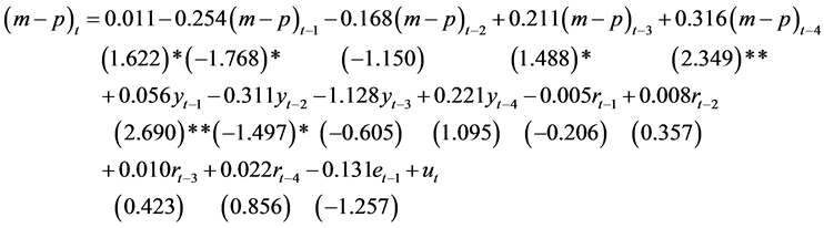 (5)
(5)
[t-statistic in parenthesis. ** and * denote significance at the 5% and 10%, respectively.]
R2 = 0.596 F = 6.932 S. E. of Regression = 0.046 The above results show that the impact of a change in real income is significantly different from zero, while the coefficients associated with interest rates are not. The coefficient attached to the error correction term  is −0.131 and is less than 1 in absolute value. However, because this latter coefficient is not statistically significant, there appears to be no adjustment toward the long-run equilibrium. This insignificance indicates that M1 money demand is not stable in the short run.
4. Concluding Remarks
This paper investigates the short-run and long-run stability properties of money demand functions in Thailand over the period of 1993Q1 to 2012Q4 using monetary aggregates. To do so it uses the Johansen cointegration test to determine whether there is a long-run relationship among the variables that comprise money demand. The findings show that cointegration exists for M1 money demand function, but not for M2 and M3 money demand function variables. Therefore, only M1 appears to play a role in the monetary transmission mechanism. Other variables (exchange rate and inflation rate) were initially included in the money demand equations, but these variables played no role as determinants of money demand in Thailand. Therefore, we exclude these variables from our reported estimates. The short-run dynamics show that real GDP is an important factor in M1 money demand, but that the interest rate is not significant. Even though there is a cointegrating relation for M1 money demand, the error-correction mechanism representing the short-run dynamics of money demand show an unstable function. This instability result implies that the use of M1 as an intermediate target to achieve an intermediate and long-run inflation rate goal might be difficult.
NOTES
1However, Goldfeld admits that his specification can be misleading under the case of missing money.

2This specification is employed by Stock and Watson and Ball .
3The maximum number of ECM models is three, but the other two are not of interest in analyzing the money demand function in the present study.