Solution of Multi-Delay Dynamic Systems by Using Hybrid Functions ()
1. Introduction
Delays occur frequently in biological, chemical, transportation, electronic, communication, manufacturing and power systems [1] . Time-delay and multi-delay systems are therefore very important classes of systems whose control and optimization have been of interest to many investigators [2] -[5] . While modeling such phenomena naturally requires the use of various systems, in many problems, such systems can not be solved explicitly. Therefore, it is important to find their approximate solutions by using some numerical methods. In recent years, the hybrid functions consisting of the combination of the Block-Pulse functions with the Chebyshev polynomials [6] , the Legendre polynomials [7] [8] , or the Taylor series [9] [10] have been shown to be a mathematical power tool for discretization of selected problems. Among these three hybrid functions, hybrids of the BlockPulse functions with the Legendre polynomials have been shown to be computationally more effective.
Recently a new hybrid function consisting of the combination of the Block-Pulse functions with the Bernoulli polynomials is presented [11] [12] . The advantages of the Bernoulli polynomials , over shifted the Legendre polynomials are:
• The operational matrix , in the Bernoulli polynomials, has less errors than
  for shifted the Legendre polynomials for
 . This is because for
  in
in  we ignore the term
  while for
  in
in  we ignore the term
 .
.
• The Bernoulli polynomials have less terms than shifted the Legendre polynomials. For example , has 5 terms while
 , has 7 terms, and this difference will increase by increasing m. Hence for approximating an arbitrary function we use less CPU time by applying the Bernoulli polynomials as compared to the shifted Legendre polynomials.
• The coefficient of individual terms in the Bernoulli polynomials , is smaller than the coefficient of individual terms in the shifted Legendre polynomials
 . Since the computational errors in the product are related to the coefficients of individual terms, the computational errors are less by using the Bernoulli polynomials.
In the present paper, we use the hybrid functions consisting of the combination of the Block-Pulse functions and the Bernoulli polynomials to solve the MDS. The method is based on converting the MDS into a system of multi-delay integral equations through integration. To eliminate integral operations, the unknown functions and various functions involved in the equations are approximated by the hybrid function and the operational matrices are used. To this end, operational matrices of multi-delay systems for the hybrid function are given. It will be seen that the operational matrices have many zero elements and are more sparse than the Legendre polynomials. These matrices are used to reduce the solution of MDS to the solution of a system of linear algebraic equations.
The paper is organized as follows: In Section 2, we describe the basic properties of the hybrid functions of the Block-Pulse and the Bernoulli polynomials required for our subsequent development. Section 3 is devoted to the formulation of linear time-varying multi-delay systems and the proposed numerical method is applied to the MDS. And in Section 4, we report our numerical findings and demonstrate the accuracy of the proposed scheme by considering some numerical examples. Finally, Section 5 gives some brief conclusions.
2. Hybrid of the Block-Pulse Functions and the Bernoulli Polynomials
Hybrid functions , are defined on the interval
  as [11]
 (1)
(1)
where  and
and  are the order of the Block-Pulse functions and the Bernoulli polynomials, respectively. The Bernoulli polynomials of order
  are defined in [13] by

where , are the Bernoulli numbers. These numbers are a sequence of signed rational numbers that arise in the series expansion of trigonometric functions [14] and can be defined by the identity

Let  be an arbitrary element in
 , there exist unique coefficients
  such that [11]

where

and

By using Equation (2) we obtain


where 
 , and
, and  denotes the inner product. So we get

with


where  is a matrix of order
  and is given by
 (2)
(2)
Integration of the vector  defined in Equation (4) can be approximated by
 (3)
(3)
where  is the
  operational matrix for integration and is given by [11]
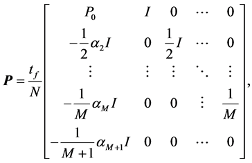 (4)
(4)
where  and
and  are the
  identity and zero matrices, respectively, and
 (5)
(5)
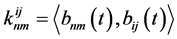
The following property of the product of two hybrid function vectors will also be used. Let
 (6)
(6)
where  is a
is a  product operational matrix. To illustrate the calculation procedure see [11] .
Multi-Delay Operational Matrix
The delay functions ,
,  are the shift of the function
  defined in Equation (4), along the time axis by
 , where
  are rational numbers in
 . It is assumed without loss of generality that
 . If we expand
  in terms of
 , we find

where  is the
  delay operational matrix of hybrid functions corresponding to
  and is given by
 (7)
(7)
where elements of the delay matrix are the  matrix
  given by
 (8)
(8)
It is noted that the first 1 in the first row is located at the  th column where

We define  as the smallest positive integer number for which
  for
for  and
and  is the greatest common divisor of the integers
 ,
, .
.
3. Problem Statement and Approximation Using Hybrid Functions
Consider the following linear time multi-delay dynamic systems:
 (9)
(9)
 (10)
(10)
 (11)
(11)
where ,
,  ,
,  and
and ,
,  , are matrices of appropriate dimensions,
  is a constant specified vector, and
  is an arbitrary known function. The problem is to find
 ,
,  satisfying Equations (13) and (14). Let
 (12)
(12)
 (13)
(13)
where  and
and  are the
  and
and  dimensional identity matrices,
  is
is  vector and
  denotes the Kronecker product [15] . Using the property of the Kronecker product,
  and
and  are matrices of order
  and
and , respectively. Assume that each
  and each of
 ,
,  ,
,  , can be written in terms of hybrid functions as

Then, using Equations (15) and (16), we have
 (14)
(14)
where  and
and  are vectors of order
  and
and , respectively, given by

Similarly, we have
 (15)
(15)
where  and
and ,
,  , are vectors of order
  given by

Let approximate  and
and ,
,  , by Equations (2)-(4) as follows
 (16)
(16)
where ,
,  are of dimensions
 , and
, and  is of dimension
 .
.
We can also write ,
,  , in terms of the hybrid functions as

where

and  is the delay operational matrix. Moreover
 (17)
(17)
 (18)
(18)
where

and

where ,
, 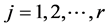 , are constant matrices of order
 . Note
  is
is  product operational matrix that to illustrate the calculation procedure we choose
  and
and . Thus we have

 (19)
(19)
where  and
and , are the
  matrices given by

By integrating Equation (12) from  to
to  and using Equations (15)-(22), we have
 (20)
(20)
simplifying Equation (23) we obtain
 (21)
(21)
by solving the set of linear algebraic equations Equation (24), we obtain the coefficients vector .
.
4. Numerical Implementation
In this section, to give a clear overview of the analysis method presented and to demonstrate the applicability and accuracy of the method three examples are given.
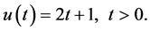
Example 1. Consider the multi-delay dynamic system from [7] described by
 (22)
(22)
with
 (23)
(23)
and
 (24)
(24)
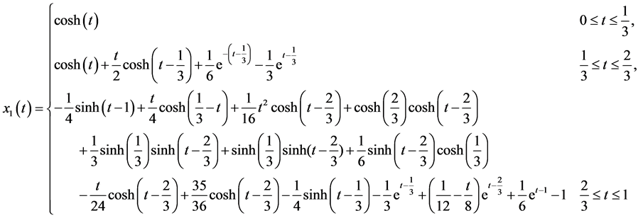
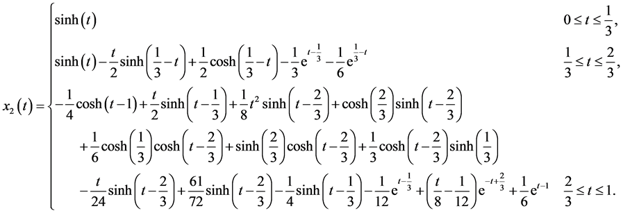
The exact solutions are
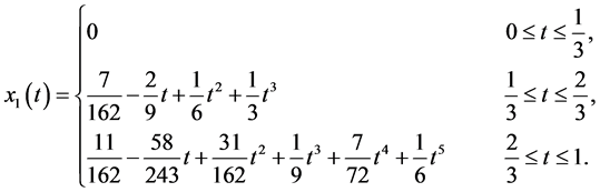

To solve this problem by the hybrid functions, we select  and
and . Let
. Let
 (25)
(25)
where ,
,  and
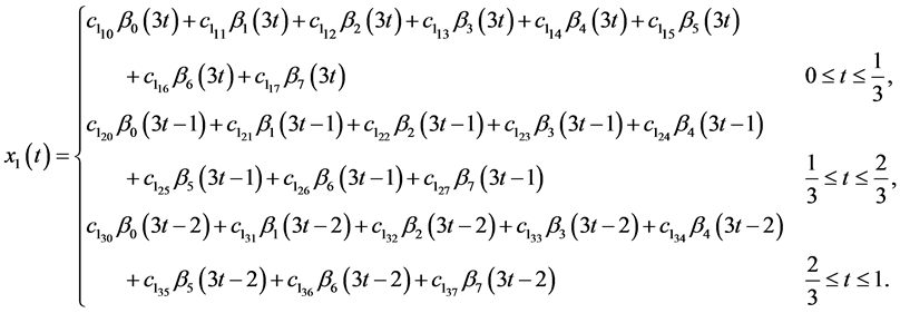
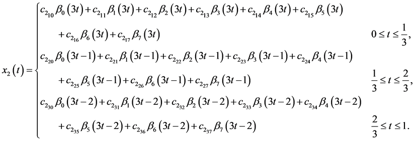
and  can be obtained similarly to Equations (3) and (4). By expanding
  and
and  in terms of the hybrid functions we get
 (26)
(26)
 (27)
(27)
Therefore, we have
 (28)
(28)
 (29)
(29)
where  and
and  the 24 × 24 matrices, can be calculated as Equation (19). Also D1 and D2 are the 24 ×24 delay operational matrices given by

where

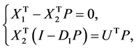
Integrating Equation (25) from  to
to  and using Equations (26)-(27) and substituting Equations (28)-(32) we get
 (30)
(30)
where  is the operational matrix of integration given in Equation (7). By solving Equation (33) the values of
  and
and  can be found as


To define  and
and  for
for  in the interval
  we map
  into
into  by mapping
  into
into , and for
  in the interval
  we map this interval into
  by mapping
  into
into , and similarly for the other intervals. From Equation (28) we get
After simplifying the same value as the exact  and
and  would be obtained.
Example 2. Consider the delay dynamic system described by
 (31)
(31)
with
 (32)
(32)
and
 (33)
(33)
The exact solutions are


To solve this problem by using of the hybrid functions, we select  and
and . Let
. Let
 (34)
(34)
where ,
,  and
and  can be obtained similarly to Equations (3)-(4). Using Equation (37) we get

where  is the
  delay operational matrix given by

where
 (35)
(35)
By expanding  in terms of hybrid functions we obtain
 (36)
(36)
Integrating Equation (34) from  to
to  and using Equations (35)-(36) and substituting Equations (37)-(39), we get
 (37)
(37)
where  is the operational matrix of integration given in Equation (7). By solving Equation (40) the values of
  and
and  can be found. By using from Equation (37) and simplifying the same value as the exact
  and
and  would be obtained.
Example 3. Consider the following multi-delay system with delay in both control and state described by
 (38)
(38)
with
 (39)
(39)
and
 (40)
(40)
The exact solutions are
To solve this problem by using the hybrid functions, we select  and
and . Let
. Let
 (41)
(41)
where ,
,  and
and  can be obtained similarly to Equations (3) and (4). By expanding
  and
and  in terms of hybrid functions we get
 (42)
(42)
Using Equation (44) and (45) we obtain
 (43)
(43)

where  and
and  are the
  delay operational matrices given by
 (44)
(44)
where

By integrating Equation (41) from 0 to t and using Equations (42) and (43) and substituting Equations (44) and (47), we get
 (45)
(45)
where  is the operational matrix of integration given in Equation (7). By solving Equation (48) the values of
  and
and  can be found. By using from Equation (44) and simplifying the same value as the exact
  and
and  would be obtained. In Table 1 a comparison is made between the exact solution and the approximation solution of
  and
and  for
for . The approximation value of
  and
and  on
on , is the same as the exact solution.
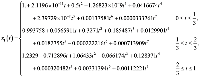


Table 1. Approximate solutions and exact solutions of Example 3.
5. Conclusion
The hybrid of the Block-Pulse functions and the Bernoulli polynomials and the associated operational matrices of integration and delay are applied to solve the linear multi-delay dynamic systems. The method is computationally very attractive, at the same time keeping the accuracy of the solution. It is also shown that the hybrid functions provide exact solutions in each subintervals for Examples 1, 2 and 3. The presented method reduces multi-delay systems to the solution a system of algebraic equations, and so the calculation is easy. The matrices ,
,  and
and  in Equations (5), (7) and (10) are sparse, hence the present method is very attractive and reduces the CPU time and computer memory.
NOTES
*Corresponding author.