1. Introduction
In quantum mechanics, the class of potentials for which Schrödinger equation can be exactly solved has been extended considerably by using different methods. The popular and widely one used in quantum mechanics is the perturbation theory leading to solve the problems approximately. Furthermore, among problems that can be exactly solved, there are few whose solutions can be obtained exactly by summing up the perturbation series in the path integral formalism [1] . Exact Green’s functions: for delta-function [2] -[4] , for Coulomb potential [5] -[7] , for the inverse square potential [8] and for the step potential [9] are obtained by summing up the perturbation series in the path integral framework. In [2] , the Feynman perturbation series are used to study the one-dimensional delta-function potential, where the authors extracted only correct informations for wave functions but they did not give the exact expression form of the propagator. The use of the same technique, perturbation series, gave the exact expression for the propagator for the delta-function potential [3] . We can find several examples of potentials problem with a delta-function perturbation by means of path integrals [4] , the Green’s function for each problem is derived by summing the Feynman perturbation series. In [5] , the perturbation series are used to derive the Green’s function for the Coulomb potential in a closed analytical form. The Green’s function of the one-dimensional relativistic Wood-Saxon, step and square well potential are evaluate by the Kleinert’s path integral technique [6] and in [7] the same author has calculated the Green’s function of the D-dimensional Coulomb by summing exactly the perturbation series; the energy spectra and wave functions are extracted. The exact propagator is derived by summing the Feynman perturbation series for a particle moving in the inverse square potential [8] . The Green’s function for the step potential is given by the exact summation of the perburbation series [9] .
The Morse potential is one of the important potentials in physics, which raises many interests in many areas specialy in molecular physics and is used for the description of the interaction between the atoms in diatomic molecules. The Schrödinger equation for the Morse potential has been solved exactly or studied by different methods recently, for example, [10] -[18] .
In the paper [19] , we have derived the Green’s function of the Morse one-dimensional potential using the perturbation series, not by summing exactly the series but we use its termes to the final result. The news is that we have presented the use of the Fourier transform in the Feymann path integral perturbation series method.
In this work, we will use the same technique in [19] and some results of the ordinary differential equations of the second ordre. We calculate the Green’s function of the problem by computing the exact sum of the perturbation series, but in a different way as in [19] .
2. Path Integral for the Morse Potential via the Sum of the Perturbation Series
We are interested to calculate the propagator, say the Green’s function relative to the one-dimensional Morse potential:

which can be written as:
 (1)
(1)
where  is the strength of the potential. The Feynman propagator is defined, taking
 , by:
, by:
 (2)
(2)
where  is the Lagrangian of the problem and
  is the formal measure on the path space. If we split the Lagrangian into the free part and the interaction part as (in unit mass):
 (3)
(3)
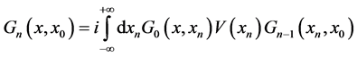
We can show that the Feynman propagator takes the form:
 (4)
(4)
where:
 (5)
(5)
And  is the free particle propagator given by:
 (6)
(6)
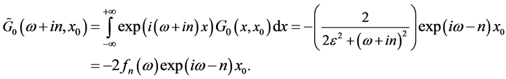
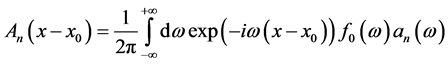
Taking the Fourier transform of  on
on  as:
as:
 (7)
(7)
we write this last formula as:
 (8)
(8)
where:
 (9)
(9)
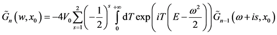
and using Equations (1) and (9), then (8) becomes:


(10)
we take now the Fourier transform on the end point  in the last formula, and using the convolution theorem for Fourier transform, we get:
 (11)
(11)
i.e.
 (12)
(12)
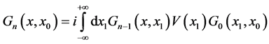
where:
 (13)
(13)
and
 (14)
(14)
From Equation (12), we see that all termes  are known and depend on the expression of
  which is:
 (15)
(15)
where we note  by:
by:
 (16)
(16)
Let now compute the first and the second terms of Equation (12):

and

and so on, we can see that all terms  are determined in a linear combination of
  and powers of
  Since
Since  is:
is:

and if we bring together all terms in power of  , we get:
 (17)
(17)
where the coefficients  satisfy the recurrence formula:
 (18)
(18)
or:
 (19)
(19)
with .
.
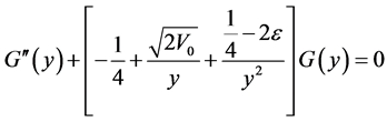
Now noting the series in Equation (17) by:
 (20)
(20)
we can easily check that  which is the generating function of
  satisfies the differential equation:
 (21)
(21)
Here we have to note that this equation is equivalent to those governing Green’s function itself but written in an other form where we have put  and done the Fourier transform on the end point
  , i.e.:
 (22)
(22)
Return now to Equation (17) and if we take the inverse Fourier Transorm on  , we obtain:
 (23)
(23)
Then if we note by:
 (24)
(24)
we see that:
 (25)
(25)
and with the Fourier transform properties, we have:
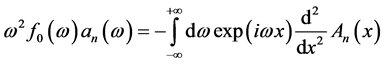 (26)
(26)
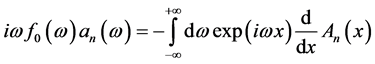 (27)
(27)
Then from these last formulas and the recurrence formula of  (19) we conclude that
  satisfies:
 (28)
(28)
with  and
and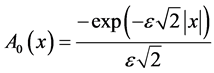 , which is a linear second order ordinary differential equation with real constant coefficients. Then
  can be expressed in term of the complementary solution plus a particular solution. Indeed, the complementary solution
  is:
is:
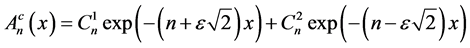 (29)
(29)
where the coefficients  and
and  are constants independent of
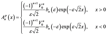
  and using the variation of parameters method we find that the particular solution has the following expression:
 (30)
(30)
with  are determined by:
 (31)
(31)
 (32)
(32)
where

Finally by recurrence, we can prove that:
 (33)
(33)
where the coefficients  satisfy an recurrence formula as:
 (34)
(34)
with  .
.
Then from Equations (29) and (33) we have:
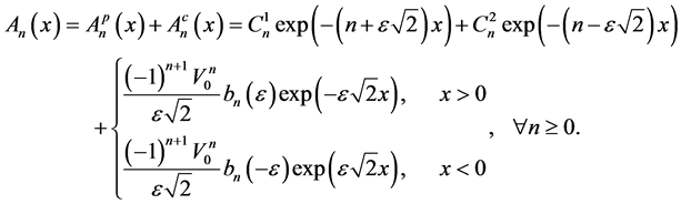 (35)
(35)
we have to note that .
.
Knowing that if the following limits exist:

then


So in that case and from the formulas (35), (25), we are able to write the Green’s function  as:
as:
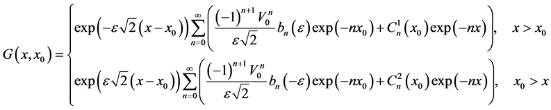 (36)
(36)
Knowing that the generating functions of  and
and  respectively are:
 (37)
(37)
then if we use the recurrence formula (34) it’s easy to deduce that these generating functions are given by:
 (38)
(38)
where  is the solution of Whittaker equation:
 (39)
(39)
and they satisfy respectively the following differential equations:
 (40)
(40)
 (41)
(41)
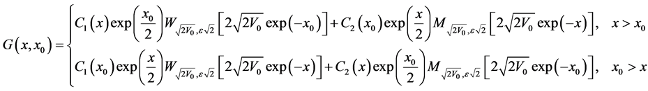
hence we can conclude that the Green’s function  takes the form:
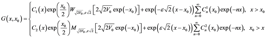 (42)
(42)
where  are the Whittaker’s functions. We draw attention here that in this last formula we have taken the Whittaker’s function
  in the case
  because it’s not singular at
 , and when
  we have taken
  which is not singular at
 . Let us now to go back to (8) i.e.:

for which it’s obvious that:
 (43)
(43)
from this formula and with the same way as above, if we take the Fourier transform on initial point  we can see that
  have another form as:
 (44)
(44)
then from Equation (42) and this last formula (44) we have for :
:
 (45)
(45)
and
 (46)
(46)
for which Equation (44) i.e.  becomes:
(47)
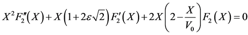
Knowing that  is a solution of the differential Equation (40), then it’s easy to check that
 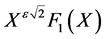 is a solution of the following differential equation:
 (48)
(48)
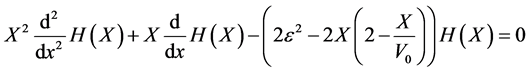
which is the same as the following differential equation:
 (49)
(49)
for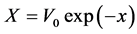 . Then we conclude that:
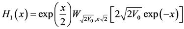
and
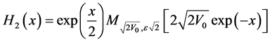
which are two linearly independent solutions of Equation (49), and since  is also solution of the differential Equation (13) for
 , form Equation (47) we can deduce that:
 (50)
(50)
and
 (51)
(51)
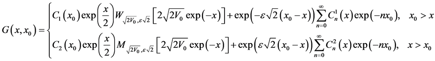
Finally we get that the Green’s function for Morse potential takes the form:
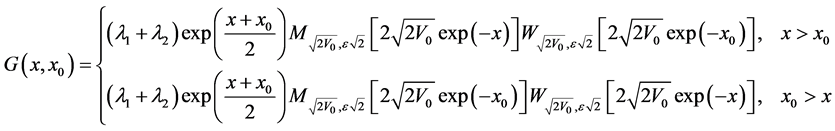 (52)
(52)
and since  is also a solution of the differential Equation (49) for
  or
or  then the Green’s function takes the form:

where  denotes Heaviside’s unit step function. A result was found earlier by different methods [11] -[13] .
3. Conclusion
In this work, we have calculated the Green’s function for the Morse potential using the perturbation method in the path integral formalism. This contribution concerns, for the first time, the calculation of the energy Green’s function of the system by summing exactly the perturbation series with the introduction of the Fourier transform and some results concerning the Green’s function of the ordinary differential equations of the second ordre. We will consider a generalization of this method specialy for other special potentials in the exponential form.