1. Introduction
Multiphase flow problems occur in a variety of scientific and technical disciplines ranging from environmental research to modeling of operations in nuclear, chemical or processing engineering installations and combustion systems. The modeling and simulation of these flows are one of the complex and challenging subjects of computational fluid dynamics (CFD). In such problems the flow regime of interest contains two or more non-mixed fluids separated by sharp interfaces. A challenging part in the numerical simulation of these models is the coupling of interface with the fluid flow model, because a coupling miss-match may introduce large errors in the numerical simulations.
Several two-phase flow models exist in the literature for describing the behavior of physical mixtures. These models use separate pressures, velocities, and densities for each fluid. Moreover, a convection equation for the interface motion is coupled with the conservation laws of flow models. In the literature such models are known as seven-equation models. One of such models for solid-gas two-phase flows was initially introduced by Baer and Nunziato [2] and was further investigated by Abgrall and Saurel [3,4], among others. The seven-equation models are considered as well-established two-phase flow models. However, such models inherit a number of numerical complexities. To resolve such difficulties researchers have proposed reduced models ranging from three to six-equation models [5-7].
The Kapila’s five-equation model [5] derived from Baer and Nunziatoseven-equation model [2] is a wellknown reduced model and has been successfully implemented to study interfacing compressible fluids, barotropic and non-barotropic cavitating flows. The model contains four conservative equations, two for mass conservation, one for total momentum and one for total energy conservation. The fifth equation is non-zero convection equation for volume fraction of one of the two phases.
Although, this five-equation model is simple, it involves a number of serious difficulties. For example, the model is non-conservative and, hence, it is difficult to obtain a numerical solution which converges to the physical solution. In the presence of shocks, the volume fraction may become non-positive. Another issue is related to non-conservative behavior of the mixture sound speed which is governed by the Wood formula [8].
To avoid such difficulties of five-equation model, Saurel et al. [1] introduced pressure non-equilibrium terms which are already present in the seven-equation model of Baer and Nunziato [3]. This reduced model is six- equation model incorporating single velocity, two pressures and relaxation terms of two-phases. An additional seventh equation, describing the total mixture energy, is added to the model which guarantees the correct treatment of the shocks in the single phase limit. Some salient features of this extended model are that it is hyperbolic with only three wave propagation speeds and the volume fraction remains positive. In [1], the authors used Godunov-type method equipped with acoustic solver and HLLC-type solver. In addition a pressure relaxation procedure is implemented to fulfill the inter face conditions.
Kinetic flux-vector splitting (KFVS) schemes have been successfully used for numerically studying flows in gas dynamics. In [9] KFVS scheme is used to solve bump in a channel problem on structured meshes. Numerically, it was found in [9] that the explicit flux function of KFVS scheme, by employing collisionless Boltzmann transport equation, is similar to the flux function of van Leer [10]. The same result was first obtained by [11]. Moreover, a high order KFVS scheme for the simulation of several two-dimensional problems on structured and unstructured meshes is in [12]. Recently, authors in [13] and [14] have constructed an improved BGK-type KFVS scheme which also incorporates particle collisions at the cell interfaces. Furthermore, [15] and [16] used different KFVS schemes for solving shallow water equations. Very recently, in [17] KFVS schemes are employed to solve a reduced five-equation two-phase flow model.
In this work, the six-equation model of Saurel et al. [1] is numerically investigated. Our primary objective is to develop a robust and efficient numerical method which is also easy to implement. A kinetic flux vector splitting (KFVS) scheme is proposed for solving this model. The suggested scheme is based on the splitting of macroscopic flux functions of the equations of two-fluid flow model. The upwinding bias in the numerical flux function can be naturally obtained by considering a fluid as a collection of particles. The movements of particles in forward or backward directions automatically split the fluxes of mass, momentum and energy into forward and backward fluxes across the cell interfaces, i.e.

where  represents a vector of mass, momentum and energy densities inside the cell
 . In this scheme, we start with the cell averaged initial data of conserved variables and get back their cell averaged values in the same cell at the next time step. In order to get second-order accuracy, MUSCAL-type initial reconstruction and Runge-Kutta time stepping method are employed.
For validation, the numerical results of KFVS scheme are compared with those obtained from the centralupwind scheme [6]. The basic idea of such schemes is that they use information of local propagation speeds and estimate the solution in terms of its cell average. Further, such schemes have an upwind nature, since they take care of directions of wave propagation by measuring the one-sided local speeds. Moreover, to further authenticate our results, HLLC-type Riemann solver [18] is also implemented to the current model.
This article is organized as follows. In Section 2, the one-dimensional single velocity and two pressures two-phase flow model is presented. Afterwards, in Section 3 the one-dimensional KFVS scheme is derived for the numerical approximation of this model. In Section 4, the one-dimensional central-upwind scheme is briefly introduced. Section 5 deals with the pressure relaxation procedure and correction step. In Section 6, some numerical test problems are presented to validate the numerical results. Finally, Section 7 gives conclusions and remarks.
2. Mathematical Model
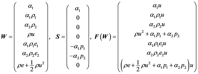
In this section, a single velocity six-equation two-phase flow model is presented [1]. This model was obtained from [2] by considering the asymptotic limit of stiff velocity relaxation. However, the non-equilibrium pressure terms are kept in the model. The six-equation model has some features which are the basic requirements for the numerical approximation of hyperbolic type systems. For example, the positivity of volume fraction and monotonic property of the mixture sound speed. In one space dimension, the six-equation model without heat and mass transfer is given as [1]:
 (1a)
(1a)
 (1b)
(1b)
 (1c)
(1c)
 (1d)
(1d)
 (1e)
(1e)
 (1f)
(1f)
Here,  is the mixture density,
  is the velocity,
  is the mixture pressure and
  is the volume fraction of phase
 . The mixture total energy
  is given as
 , with mixture internal energy e is defined by
 (2)
(2)
where 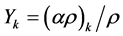 is the mass fraction for phase k. Further, the mixture density is define by
 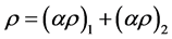 , where according to stiffened gas equation of state (EOS)
 (3)
(3)
Here,  and
and  are material specific constants of the fluid. From Equation (2) one can find the mixture pressure
  as under
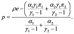 (4)
(4)
Here,  is the interfacial pressure which is defined as
 (5)
(5)
where  is the acoustic impedance of phase
 . The combination of the two internal energy equations with mass and momentum equations in Equation (1) give an additional mixture energy equation additional equation for the mixture energy
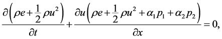 (6)
(6)
where  .
.
As the model (1) is non-conservative, the non-conventional jump conditions are required for the convergence of numerical methods which are based on Reimann solver. These jump conditions are derived in [1] for HLLC scheme. It is worth mentioning that the proposed KFVS and central-upwind schemes do not require such jump conditions.
As it is mentioned earlier that the model under consideration has an attractive feature regarding the mixture sound speed, the mixture sound speed behaves monotonically against mass and volume fractions and is called as the frozen sound speed. It is defined as
 (7)
(7)
where the phasic sound speed  is given as
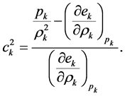 (8)
(8)
The Equation (1a) can be written in the following form
 (9)
(9)
In view of Equations (1) and (9), the model (1) can be rewritten as
 (10a)
(10a)
where
 (10b)
(10b)
The term  in the volume fraction equation and the terms
  in the two energy equations for
 are treated in the same manner as the flux vector terms.
To close the system (1) and (6), additional equations are needed. In the present case, it is assumed that each phase is described by the stiffened gas EOS given by Equation (3).
3. The KFVS Scheme
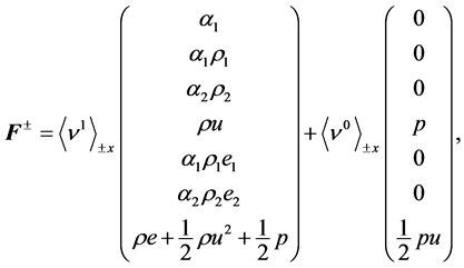
In this section, the KFVS scheme is implemented to solve the system of Equations (1) and (6). In gas-kinetic theory, the flux is related to the particle motion across a cell interface. The numerical discretization of the current system corresponds to the evaluation of local macroscopic flux-vector  through each boundary of the mesh cell. The particle motion in the x-direction determines the flux function. The remaining quantities, such as densities, pressure and volume fraction can be considered as passive scalars transporting with the particle velocity. Normally, particles are randomly distributed around the average velocity.
In statistical mechanics, the local Maxwellian distribution function is used to describe the distribution of moving particles along coordinate directions. The Maxwellian distribution function  in the normal direction
  is given as (e.g. [14])
 (11)
(11)
where ρ and p are mixture density and pressure. In the one-dimensional case . The transport of any flow quantity is due to the movement of particles. Thus, in the one-dimensional case, with the distribution function
  given by Equation (11) one can split the particles into two groups. One group is moving to the right with positive velocity
  and the other group is moving to the left with negative velocity
 . Before splitting the fluxes, let us define
 (12)
(12)
 (13)
(13)
The above two moments are sufficient to split all the fluxes. The zeroth order moment (12) is used to split scalars while the first order moment (13) is used for vectors. In order to simplify the notation, we define
 (14)
(14)
 (15)
(15)
and
 (16)
(16)
 (17)
(17)
In the above equations, the positive sign represents those particles moving in the positive (right) direction and the negative sign represents the particles moving in the negative (left) direction. Moreover, the complementary error function is defined as
 (18)
(18)
With the help of above flux-splitting technique, we can derive a KFVS scheme for solving the system of Equations (1) and (6).
In order to apply a finite volume scheme, the first step is to subdivide the domain of interest into  subdomains or mesh cells. Let us define the cell
  by interval
  for
for Therefore,
 represents the uniform cells width, the points
  refer to the cells center and the points
 represent the cells faces. We start with a cell averaged initial data
  at time step
  and compute the cell average updated solution
  over the same cells at the next time step
 . This is performed easily by assuming the CFL condition
 (19)
(19)
where  is the speed of sound defined in Equation (3). With the help of above defined setup we can split the flux functions of the six-equation model in Equation (10) as
 (20)
(20)
where
 (21)
(21)
where . Here, the flux-vector at the right interface of the cell
  is given as
 (22)
(22)
Analogously, we can define the left interface flux-vector of the cell . The integration of the Equation
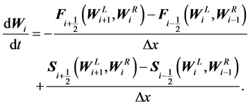
(10) over the cell  gives the following semi-discrete kinetic upwind scheme
 (25)
(25)
Here, we have assumed the cell averaged values of the non-differential source term . The cell averaged values
 are defined as
 (24)
(24)
Similarly,  can be defined and
  are given by (22). Moreover,
 (25)
(25)
The splitting procedure in Equation (25) is analogous to that presented in (20)-(22) for cell interface fluxes.
The above scheme is first order accurate in space. To achieve high order accuracy, the initial reconstruction strategy must be applied for interpolating the cell averaged variables . Here, a second order accurate MUSCL-type initial reconstruction procedure is employed. Starting with a piecewise-constant solution,
  , one can reconstruct a piecewise linear (MUSCL-type) approximation in x-directions by selecting the slope vector (differences)
 . The boundary extrapolated values are given as
 (26)
(26)
A possible computation of these slopes, is given by family of discrete derivatives parameterized with , for example
 (27)
(27)
where  is a parameter and
  denotes central differencing
 (28)
(28)
Here  denotes the min-mod non-linear limiter
 (29)
(29)
On the basis of above reconstruction procedure, a semi-discrete high resolution kinetic solver is given as
 (30)
(30)
To obtain second order accuracy in time, we use a second order TVD Runge-Kutta scheme to solve (30). Denoting the right-hand side of (30) as , a second order TVD Runge-Kutta scheme update
  through the following two stages [13]
 (31a)
(31a)
 (31b)
(31b)
where  is a solution at previous time step and
  is updated solution at next time step. Moreover,
  represents the time step.
4. Central-Upwind Scheme
In the literature central schemes are regarded as suitable numerical tools to approximate the hyperbolic conservation laws. In this work, to validate the numerical results of KFVS scheme, the central-upwind scheme is for the first time applied to solve the given model [19].
This scheme belongs to the new family of central schemes introduced by Kurganov and Tadmor [19]. The core concepts behind the development of such schemes are the use of information of local propagation speeds and estimate the solution in terms of its cell average. Moreover, these schemes have an upwind nature, since they respect the directions of wave propagation by measuring the one-sided local speeds. Due to this feature, they are called as central-upwind schemes. Here, we present the final formulation of the scheme, see [19] for further details regarding the scheme derivation. In semi-discrete form the scheme is given as [19]
 (32)
(32)
where  is the numerical flux defined by
 (33)
(33)
The intermediate values  and
and  are given by Equation (26). Here,
  represents the maximal local speed which in the generic case could be
 (34)
(34)
Moreover,  and
and .
.
5. Pressure Relaxation Procedure
The pressure relaxation plays a vital role to fulfill the interface conditions. Here, the pressure relaxation procedure of Saurel et al. [10] is used. For this purpose, we have to solve the following system, which is obtained by applying the Strang splitting approach [20] to the system (1) and (6), i.e.
 (35a)
(35a)
 (35b)
(35b)
 (35c)
(35c)
 (35d)
(35d)
 (35e)
(35e)
 (35f)
(35f)
 (35g)
(35g)
where .
.
Using the volume fraction Equation (35) with mass Equations (35b) and (35c), the internal energy Equations (35e) and (35f) can be written as under
 (36)
(36)
where  is the mass fraction of phase
 . Integration of these equations results in the following approximations
 (37)
(37)
Here, the super scripts “0” and “*” indicate the values of the variables before and after relaxation process, respectively. To approximate the average interface pressure, the following estimates can be used
 (38)
(38)
where  is the relaxed pressure. However, as mentioned in [10], the choice of this approximation has no significant effect on the computations.
Clearly, Equation (37) comprises of two equations. But, there are three unknowns ,
,  and
and . To close the system we need an extra equation, which could be the saturation constraint
 (39)
(39)
But

because  are constant during the relaxation process. Therefore, Equation (39) can be written as
 (40)
(40)
Using the EOS in Equation (3) into Equation (37) the specific volume can be expressed as
 (41)
(41)
Now, using Equation (41) into (40), we get single equation with only one unknown 
 (42)
(42)
To find the relax pressure, the Newton’s method is used. After having the relax pressure, the specific volume and volume fractions for two phases can be found.
Correction Step
Since the volume fractions have been approximated through relaxed pressure. The mixture pressure can be obtained from Equation (4)
 (43)
(43)
The mixture pressure in Equation (4) is obtained from the evolution of the mixture total energy in Equation (6). As the energy equation is in conservative form, therefore, it is expected to be valid in the entire flow field. Thus, the mixture pressure is used with EOS for each phase to reset the value of the internal energies.
6. Numerical Test Problems
In this section, three one-dimensional numerical test problems are presented to validate the results obtained by the application of KFVS and central-upwind schemes to six-equation two-phase flow model. For comparison, we have used the HLLC-type Riemann solver [1].
6.1. Sod’s Problem
This problem is similar to the Sod’s problem in the single phase gas dynamics. In this problem, the density and pressure ratios are large and the left and right gases have different ratios of specific heats. Both gases are separated by a very thin membrane placed at  and are initially at rest. The left side gas has high density and pressure compared to that on the right side of the membrane. After removing the membrane, the gases evolution in time takes place. The initial data are given as

The ratio of specific heats for the left and right side gases are taken as  and
and , respectively. The numerical results at
  are shown in Figure 1. The solution contains a left-going rarefaction wave, right-going shock wave and the right-moving two-fluid interface. In Figure 1, the solutions of KFVS and central upwind schemes are compared at
  mesh cells. The reference solution is obtained from the same central upwind scheme at 2000 grid points. Both schemes give correct location of the discontinuities and have comparable accuracy. Moreover, no pressure oscillations are observed in the solution.
Table 1 gives  -errors in the density for KFVS and central schemes for different number of grid points. It is clear from the results that KFVS scheme produces less errors in the solutions compared to the central scheme.
6.2. Shock Tube Problem
In this test problem, a shock-tube of  is considered. It is filled with a liquid under high pressure on the left and with the vapors at atmospheric pressure on the right. This test problem was also studied in [21]. The initial data are

For numerical reasons, the presence of a small volume fraction of the other fluid on both sides of the diaphragm is allowed, say . The results are computed at 1000 mesh cells with final simulation time
 . Here, ratios of specific heats are given as
  and
and . Further,
  ,
,

Figure 1. Results of problem 6.1 at t = 0.015.

Table 1. L1-Errors in the density for problem 6.1.
 ,
,  and
and .
.
The same problem was also solved by HLLC-type Riemann solver. The numerical results are shown in Figure 2. It can be observed that proposed schemes give comparable results. However, small overshoot can be observed in the results of KFVS and central schemes at the interface in the velocity profile. Overall, the results of all three schemes agree well.
6.3. Two-Fluid Mixture Problem
The initial values are given as

Here, ratio of specific heats are  and
and .
.
This problem is considered as a hard test problem for a numerical scheme. A left moving rarefaction wave, a contact discontinuity, and a right moving shock wave can be observed in the solution. The right moving shock hits the interface at . The shock continues to move towards right and a rarefaction wave is created which is moving towards left. We choose 400 mesh cells and the final simulation time is taken as
 . The numerical results are shown in Figure 3. The figures show that both schemes give comparable results. However, KFVS scheme has better resolved discontinuities in the solution.
6.4. Comparison Test Problem
In this section we study a water-air mixture to analyze and compare the results obtained from five-equation [6,18], six-equation [1] and seven-equation [4] models. The initial values of the problem are

Figure 2. Results of problem 6.2 at t = 0.000473.

Figure 3. Results of problem 6.3 at t = 0.012.

Here,  ,
,  ,
,  ,
,  ,
,  and CFL = 0.5. This problem is simulated for three models. The KFVS is implemented for five-equation model and HLLC-type Riemann solver is used for six-equation and seven-equation models. The results are computed at 200 mesh cells and the final simulation time is
 . Figure 4 shows the results for comparison of three models.
Here, the five-equation model solution is considered as the reference solution. It is observed that the solutions obtained from six-equation model do not converge while the seven-equation model results are comparatively better. Such situations may arise in extreme initial conditions in mixtures. Therefore, the schemes for six-equation and seven-equation models may give wrong shock speed and wrong jumps. This observation is also reported in [22]. Thus, further work is needed to tackle such extreme conditions.
7. Conclusion
In this article, a reduced six-equation two-phase flow model of Saurel et al. [10] was numerical investigated. The model incorporates single velocity, two pressures and relaxation terms. An additional seventh equation, describing the total mixture energy, is added to the model to guarantee the correct treatment of shocks in the single phase limit. Some salient features of the model are that it is hyperbolic with only three wave propagation speeds and the volume fraction remains positive. The high resolution kinetic flux-vector splitting (KFVS) scheme and central upwind scheme were applied to solve the given model. The KFVS is based on the direct splitting of macroscopic flux functions of the system of equations. The central upwind scheme belongs to the new family of central schemes introduced by Kurganov and Tadmor [7]. The scheme utilizes information about the local propagation speeds and estimates the solution in terms of its cell average. Moreover, the scheme has upwind nature in semi-discrete form, since it respects the direction of wave propagation by measuring the one-sided local speeds. The second order accuracy of the suggested schemes was achieved by using MUSCL-type initial reconstruction and Runge-Kutta time stepping method. Moreover, a pressure relaxation procedure was used to fulfill the interface conditions. The numerical results of the schemes were compared with each other and HLLC scheme. Both schemes showed comparable performance in the selected test problems. The accuracy, efficiency and simplicity of the KFVS and central schemes demonstrate their potential for modeling two-phase flows. This work was a first step towards the approximation of the full seven-equation model by KFVS and central upwind schemes. The seven-equation model is non-conservative and non-strictly hyperbolic. Therefore, this model gives tough time to a numerical scheme. The current experience with the reduced model will be useful to solve the full seven-equation models more efficiently and accurately. Work is in progress in this direction and will be presented soon for publication.

Figure 4. Results of problem 6.4 at t = 0.00002.
Acknowledgements
A partial support from the Higher Education Commission of Pakistan at the COMSATS Institute of Information Technology Islamabad is gratefully acknowledged.