Fast Finite Difference Solutions of the Three Dimensional Poisson’s Equation in Cylindrical Coordinates ()
1. Introduction
The three-dimensional Poisson’s equation in cylindrical coordinates  is given by
 (1)
(1)
which is often encountered in heat and mass transfer theory, fluid mechanics, elasticity, electrostatics, and other areas of mechanics and physics. In particular, the Poisson equation describes stationary temperature distribution in the presence of thermal sources or sinks in the domain under consideration.
The analytic solution for the three-dimensional Poisson’s equation in cylindrical coordinate system is much more complicated and tedious because of the complexity of the nature of the problems and their geometry, and the availability of appropriate methods. To solve Poisson’s equation in polar and cylindrical coordinates geometry, different approaches and numerical methods using finite difference approximation have been developed. For instance, Chao [1] developed a direct solver method for the electrostatic potential in a cylindrical region; Chen [2] developed a direct spectral collocation Poisson solver for several different domains including a part of a disk, an annulus, a unit disk, and a cylinder using the weighted interpolation technique and non-classical collocation points;
Christopher [3] developed a solution method in an annulus using conformal mapping and Fast Fourier Transform; Kalita and Ray [4] have developed a high order compact scheme on a circular cylinder to solve their problem on incompressible viscous flows; Lai and Wang [5] developed a fast direct solvers for Poisson’s equation on 2D polar and spherical coordinates based on FFT; Swarztrauber and Sweet [6] developed a direct solution of the discrete Poisson equation on a disk in the sense of least squares; Mittal and Gahlaut [7,8] developed high order finite difference schemes to solve Poisson’s equation in cylindrical symmetry; Tan [9] developed a spectrally accurate solution for the three-dimensional Poisson’s equation and Helmholtz’s equation using Chebyshev series and Fourier series for a simple domain in a cylindrical coordinate system; Iyengar and Manohar [10] derived fourthorder difference schemes for the solution of the Poisson equation which occurs in problems of heat transfer; Iyengar and Goyal [11] developed a multigrid method in cylindrical coordinates system; Lai and Tseng [12] have developed a fourth-order compact scheme, and their scheme relies on the truncated Fourier series expansion, where the partial differential equations of Fourier coefficients are solved by a formally fourth-order accurate compact difference discretization; Xu et al. [13] developed a parallel three-dimensional Poisson solver in cylindrical coordinate system for the electrostatic potential of a charged particle beam in a circular, which used Fourier expansions in the longitudinal and azimuthal directions, and spectral element discretization in the radial direction, and some other developments had also been observed. The need to obtain the best solution for the Poisson’s equation is still in progress.
In this paper, we develop a second-order finite difference approximation scheme and solve the resulting large algebraic system of linear equations systematically using block tridiagonal system [14] and extend the Hockney’s method [15] to solve the three dimensional Poisson’s equation on Cylindrical coordinates system.
2. Finite Difference Approximation
Consider the three dimensional Poisson’s equation in cylindrical coordinates  given by

and the boundary condition
 (2)
(2)
where  is the boundary of
  and
and  is
is

and


Consider Figure 1 as the geometry of the problem. Let  be discretized at the point
  and for simplicity write a point
  as
as  and
and  as
as .
.
Assume that there are M points along , N points along
  and P points along the
  directions to form the mesh, and let the step size along the direction of
  be
be , of
, of  be
be  and
and  be
be .
.
Here ,
,  and
and  where
where  and
and  For
For , using the central difference approximation scheme that
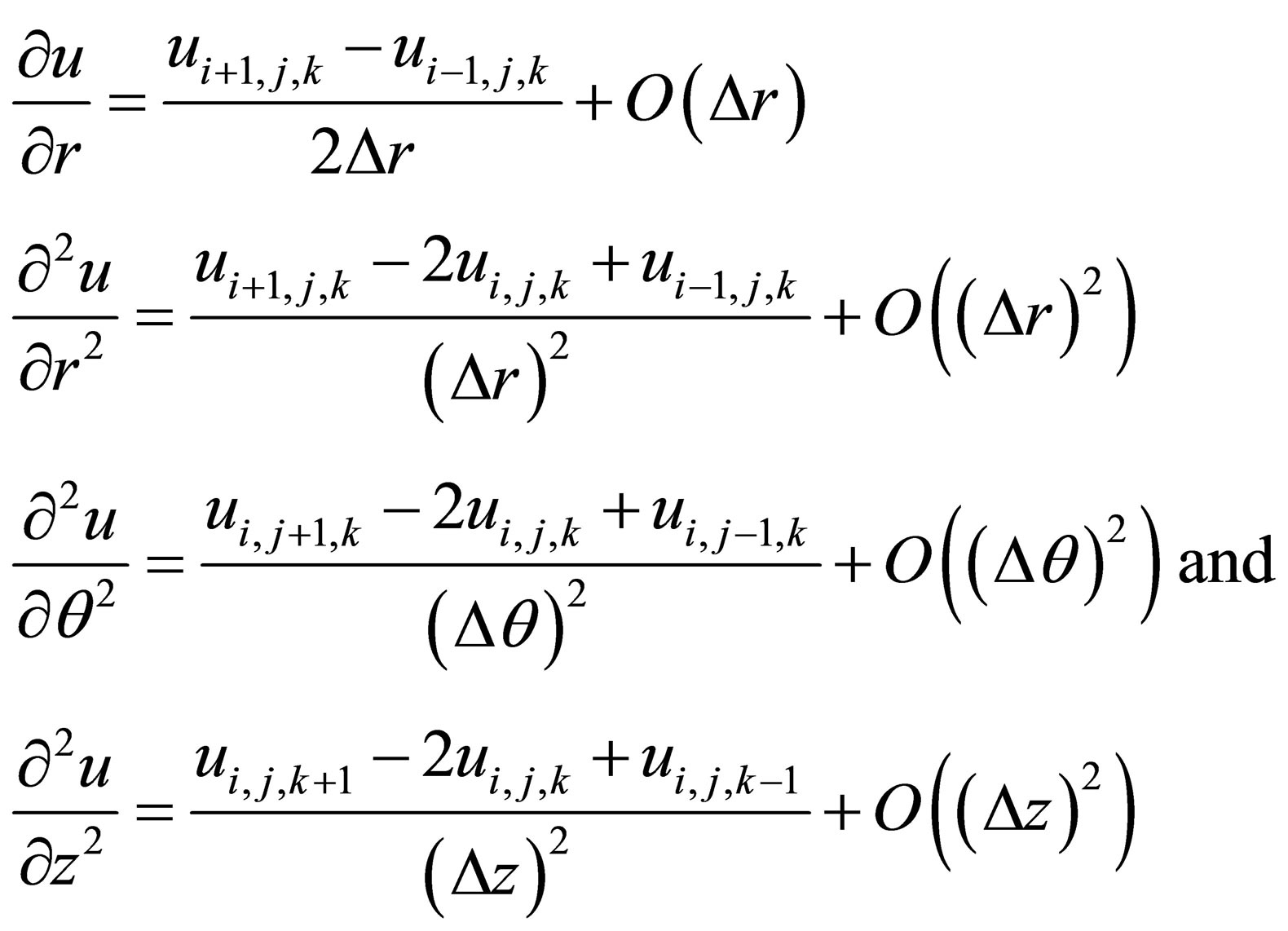 (3)
(3)
Truncating higher order differences of (3) and substituting (3) in (2), we have
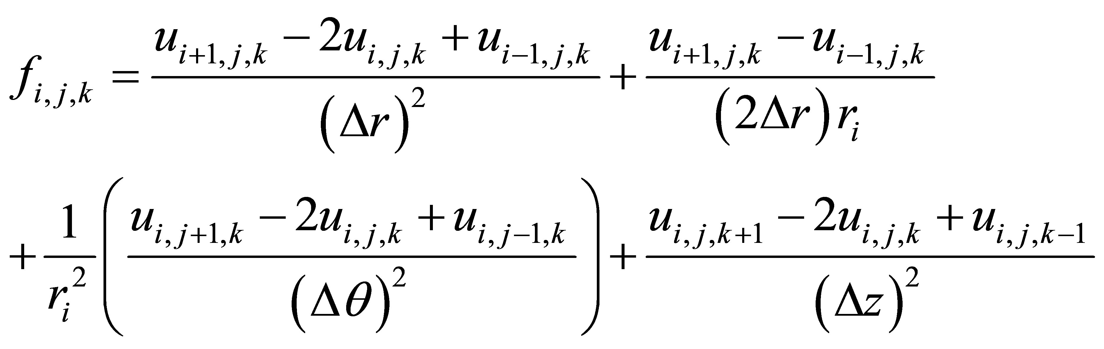 (4)
(4)
Let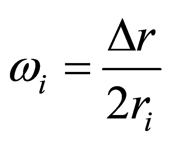 ,
,  ,
,  and
and .
.
Multiplying both sides of (4) by , rearranging and simplifying further, we get
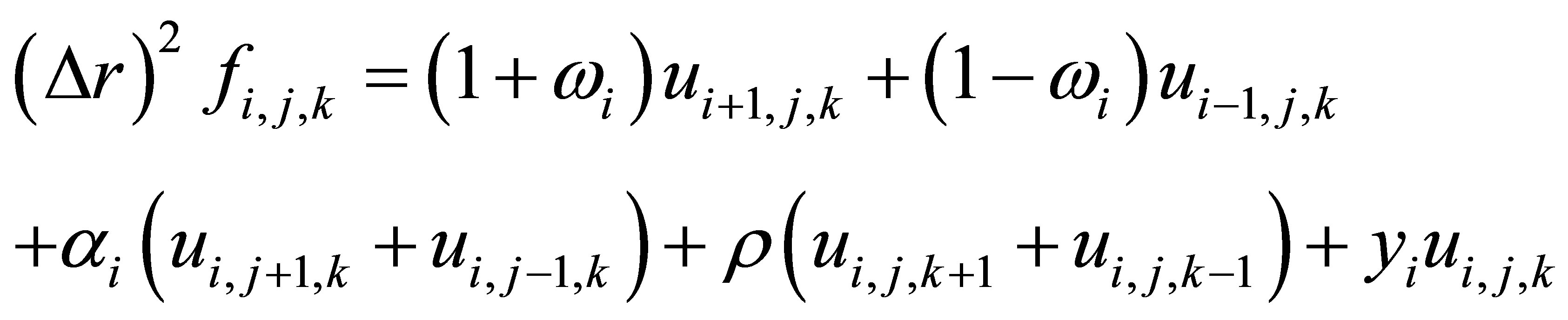 (5)
(5)
When there are two or more space dimensions the band width is larger and the number of operations goes up and thus the computation for the solution is not such an easy task.
The system of Equations in (5) is a linear sparse system, and thereby saving on both work and storage compared with a general system of equations. Such savings are basically true of finite difference methods: they yield sparse systems because each equation involves only a few variables. Now we use these advantages.
Consider Equation (5) first in the  direction, next in the
  direction and lastly in the
  direction, and hence Equation (5) can be put in matrix form as
 (6)
(6)
where 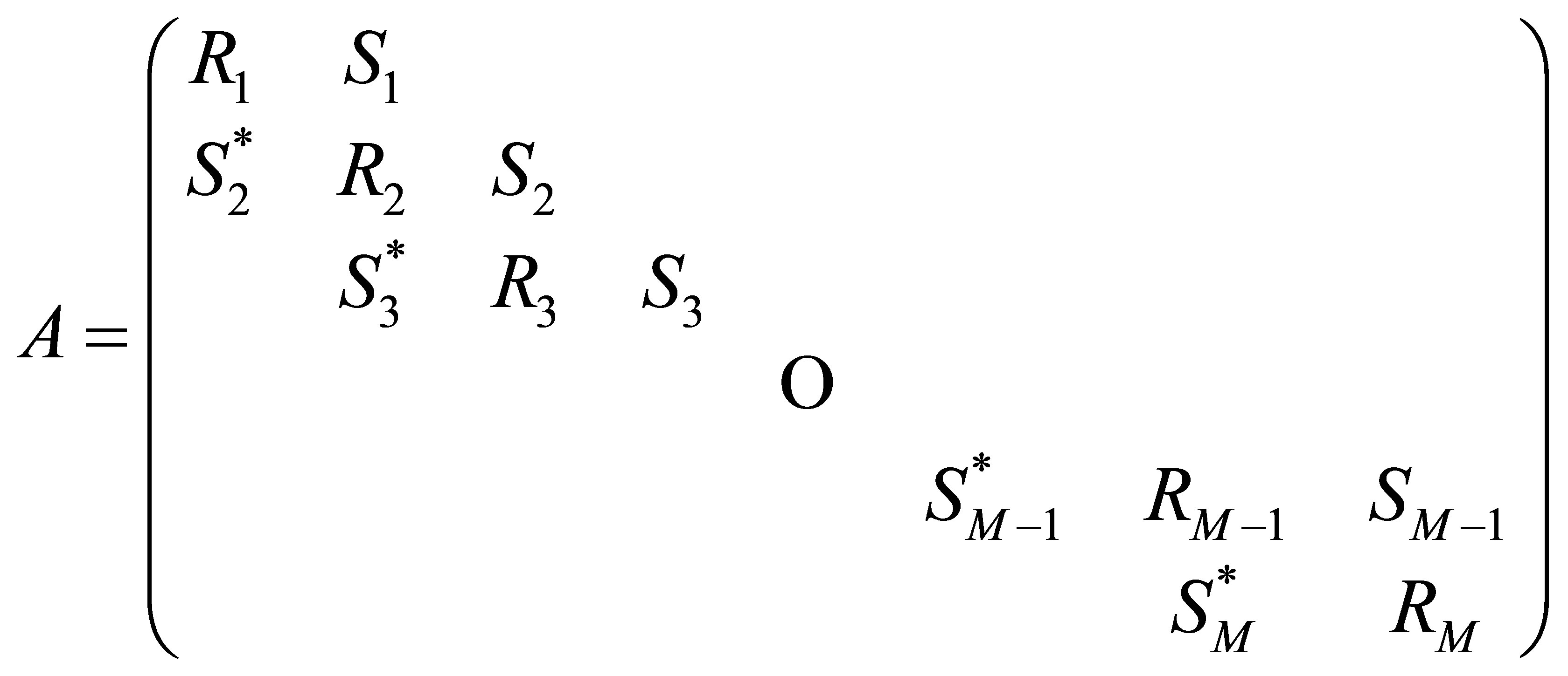
it has M blocks and each block is of order NP.
 (7)
(7)
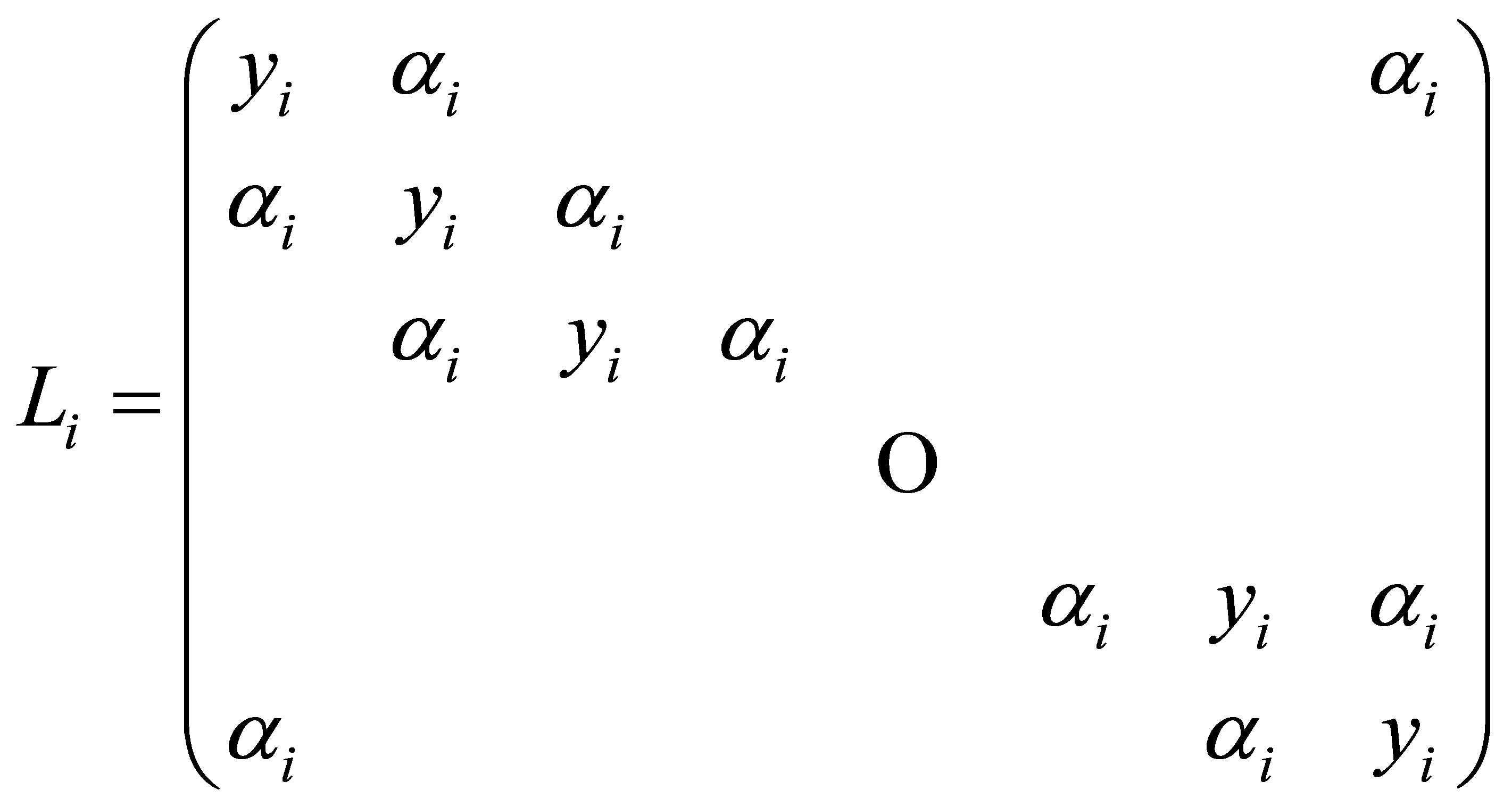
For ,
,
 (8)
(8)
For ,
,
 (9)
(9)
is a circulant matrix;
Both matrices (8) and (9) are of order N; and  is of order N.
 has P blocks and
 is of order N
 has P blocks and
 is of order N.
 ,
,
 and
and
 such that each
  represents a known boundary values of
  and values of
 , and
, and ,
,
 and
and
We write (6) a
 (10)
(10)
3. Extended Hockney’s Method
Observe that the matrix  is a real symmetric matrix and hence its eigenvalues and eigenvectors can easily be obtained.
for 
 and for

 ,
,
 .
.
Let  be an eigenvector of
  corresponding to the eigenvalue
  and the matrix
 be a modal matrix of
 ,
,
 such that
  and
and
The  modal matrix Q is defined by
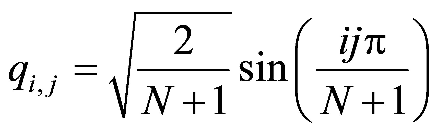 for
for  and
and
 , where
  for
for
 and
and ,
, 
Let  be a matrix of order NP.
Thus  satisfy the property that
  since
since  and due to the matrix
  is symmetric, we have
  (say);
 and
and  since both
  and
and  are diagonal matrices.
Let 
 (11)
(11)
where ,
,
 ;
;
 and
and
Pre-multiplying Equation (10) by  and applying (11), we get
 (12)
(12)
Now from each Equation of (14) we collect the first equations and put them as one group of equation
 (13)
(13)
Collect as the first set of equations by putting  in Equation (15), for
  and
and 
 and
and
 (14a)
(14a)
Again consider the second equations by putting , and get
 and
and
 (14b)
(14b)
Continuing in this manner and finally considering the last equations for , we obtain
 and
and
 (14c)
(14c)
All these set of Equations (14a)-(14c) are tri-diagonal ones and hence we solve for  by using Thomas algorithm. With the help of (11) again we get all
  and this solves (5) as desired. By doing this we generally reduce the number of computations and computational time.
4. Numerical Results
In order to test the efficiency and adaptability of the proposed method, computational experiments are done on some selected problems that may arise in practice, for which the analytical solutions of  are known to us. The computed solutions are found for any values of M, N, and P. Here results are reported at some randomly taken points from Tables 1 to 7.
Example 1. Consider  with the boundary conditions


The analytical solution is
 and the results of this example are shown in Table 1.
Example 2. Consider 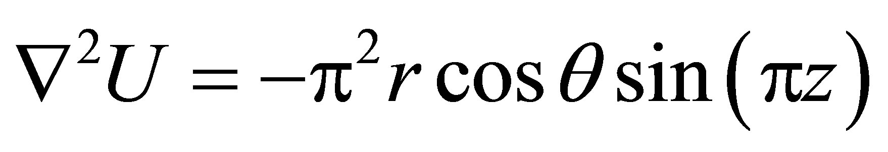 with the boundary conditions


The analytical solution is  and results of this example are shown in Table 2
Example 3. Consider
with the boundary conditions

 and
and

The analytical solution is
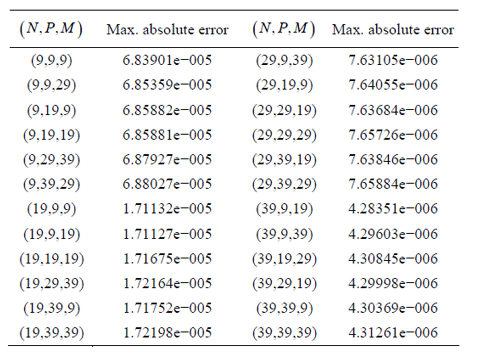
Table 1. Maximum absolute error of example 1.

Table 2. Maximum absolute error of example 2.
 and results of this example are shown in Table 3
Example 4. Consider

where 

 ,
,  and
and 
The analytical solution is

This problem was considered as one test problem by Iyengar and Goyal [11] and their result and our are found to be the same for h = 1/8, but their method cannot be applied for non-uniform values ,
,  and
and . We have shown the results of this example in Table 4.
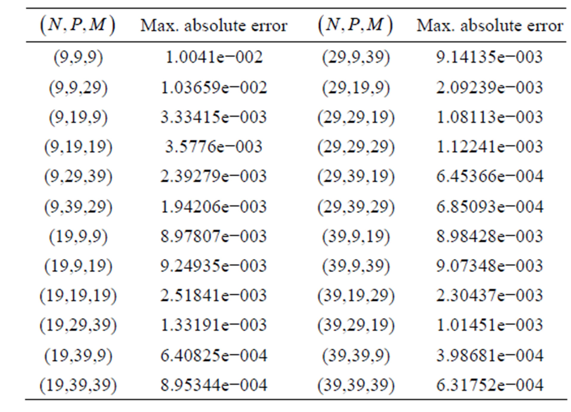
Table 3. Maximum absolute error of example 3.

Table 4. Maximum absolute error of example 4.
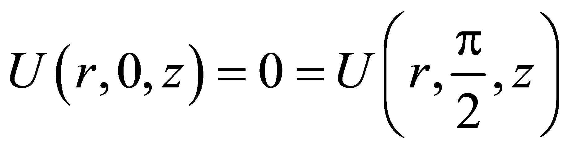
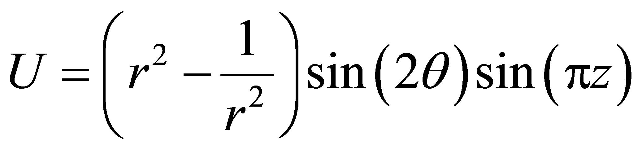
Example 5. Consider 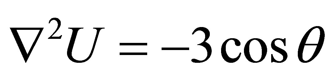 with the boundary conditions
 ,
,

The analytical solution is  and results of this example are shown in Table 5.
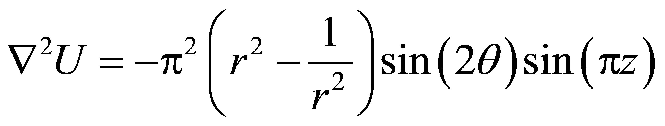
Example 6. Consider 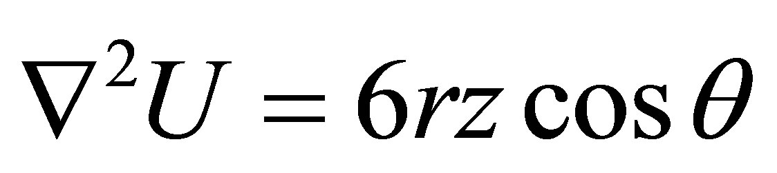 with the boundary conditions
 ,
,
 and
and 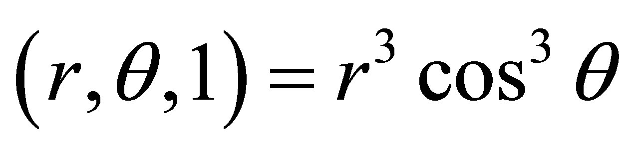
The analytical solution is  and results of this example are shown in Table 6.
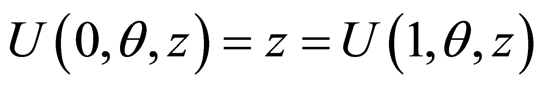
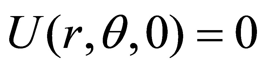
Example 7. Consider
with the boundary conditions
The analytical solution is
 and results of this example are shown in Table 7. Here, we have displayed only for some points which are taken randomly, but we can show the results at any point inside the cylinder.
5. Conclusion
In this work, first we apply Hockney’s method in order to reduce (5) as a tri-diagonal matrix and after that all the computations directly rely on the Thomas Algorithm. By
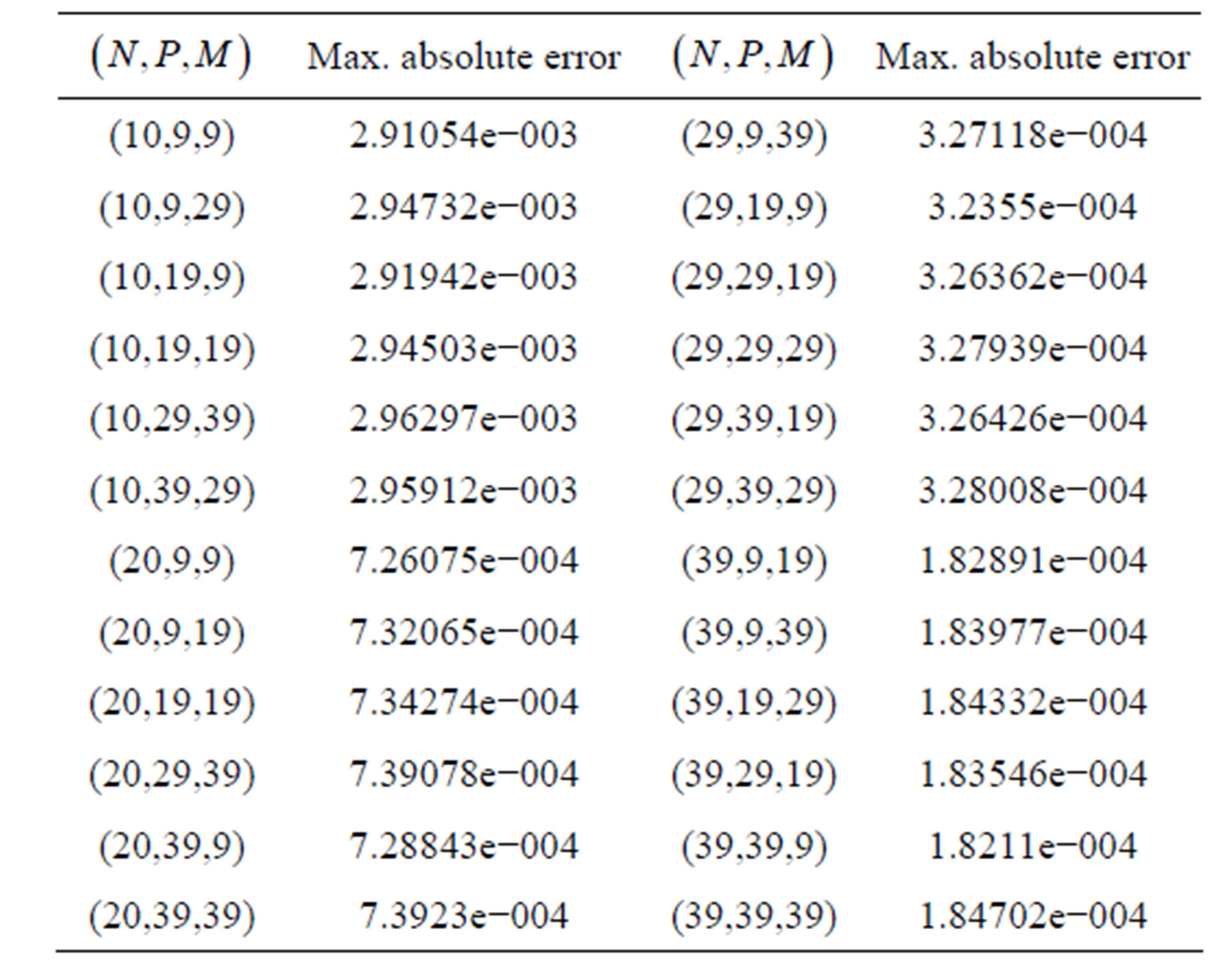
Table 5. Maximum absolute error of example 5.
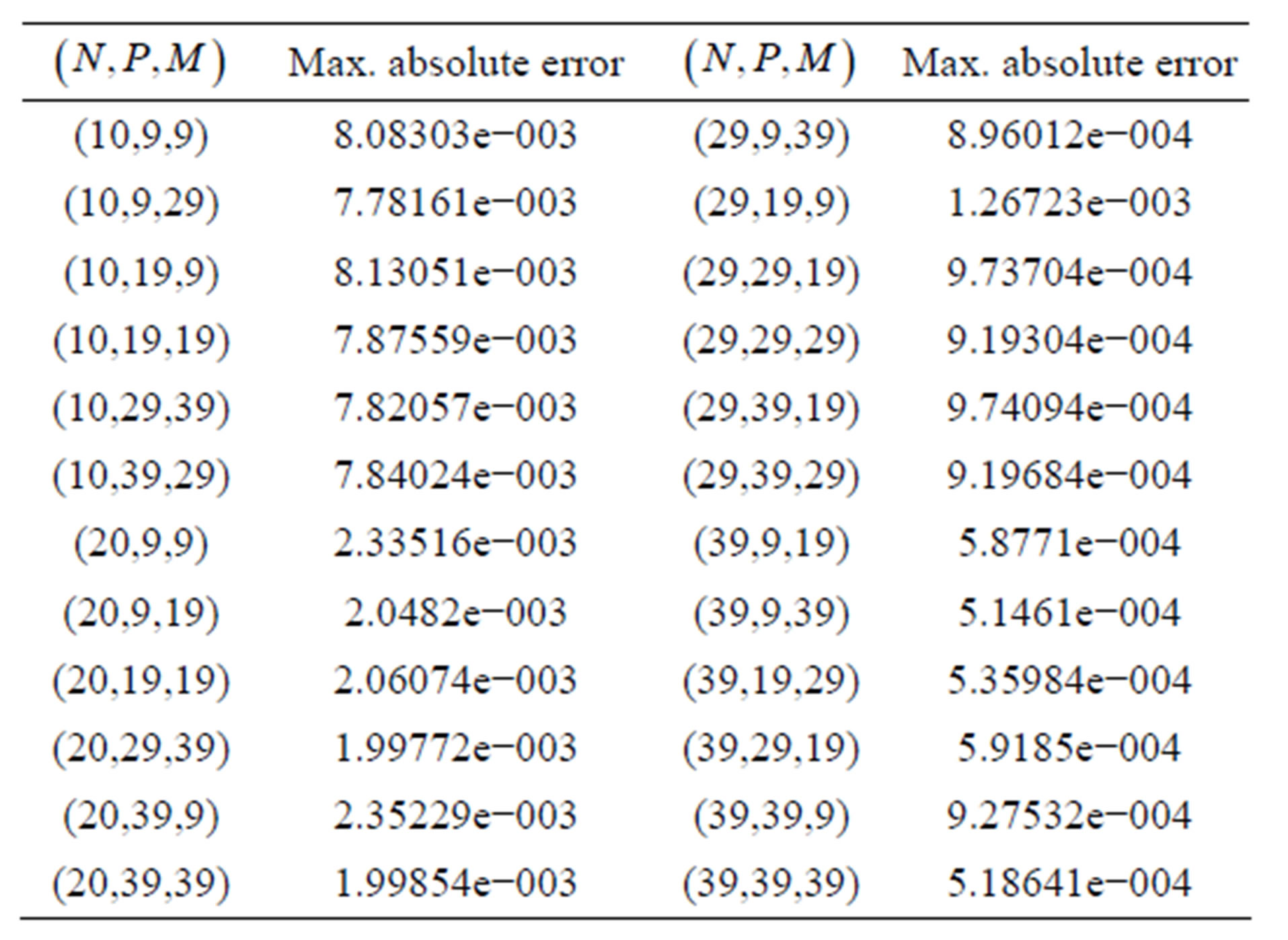
Table 6. Maximum absolute error of example 6.

Table 7. Maximum absolute error of example 7.
doing this, we saved the number of computation and computational time. The method is shown to produce good results.