Hans A. Panofsky’s Integral Similarity Function—At Fifty ()
1. Introduction
In his famous paper entitled Determination of stress from wind and temperature measurements, Hans A. Panofsky (HAP) presented a new profile function for the mean horizontal wind speed,  with
with , under the condition of diabatic stratification given by [1]
 . (1.1)
Here,  is the friction velocity,
  is the density of air,
  is the friction stress vector invariant with height,
  ,
,  , and
, and  are the components of the wind vector with respect to a Cartesian coordinate frame, where the horizontal unit vectors are denoted by
  and
and , and
, and  stands for the unit vector in vertical direction,
  is the height above ground, and
  is the (aerodynamic) roughness length. The quantity
  is HAP’s integral similarity function for momentum defined by
 , (1.2)
where  is the local similarity function for momentum according to Monin and Obukhov [2] related to the non-dimensional shear of the mean horizontal wind speed by
 . (1.3)
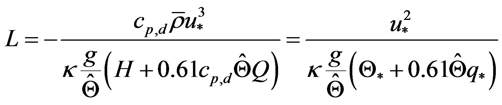
Here,  is the Obukhov number,
  is the Obukhov stability length given by
 , (1.4)
 is the von Kármán constant, g is the acceleration of gravity,
  is a potential temperature representative for the layer under study,
  is the vertical component of the sensible heat flux density (hereafter a flux density is simply denoted as a flux), and
  is the specific heat at constant pressure. The overbar denotes the conventional Reynolds’ [3] mean, and the prime, as used in Equation (1.5), the departure from that. The hat characterizes Hesselberg’s [4] density weighted mean and a double prime denotes the deviation thereof. According to Hesselberg, the density-weighted average of a quantity
  like the wind components,
  ,
,  , and
, and , the potential temperature,
  , and the specific humidity,
  , is given by
 . The difference between the conventional Reynolds mean and the Hesselberg mean can be expressed by (e.g., [5-10])
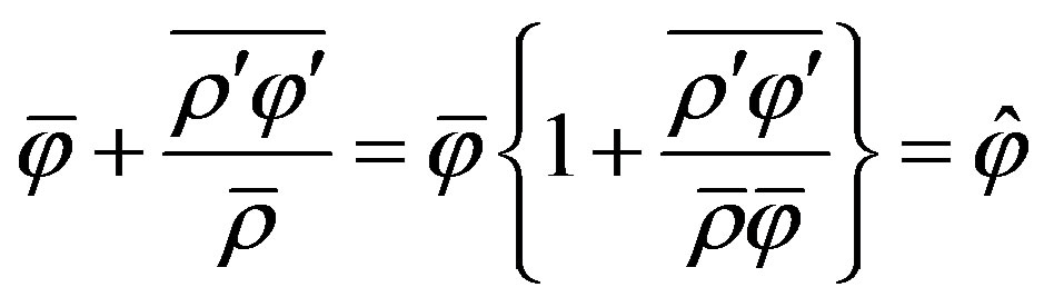 , (1.5)
where  and
and  are nearly identical if the condition
  is fulfilled.
Equation (1.3) can be derived on the basis of Buckingham’s [11]  theorem using the similarity hypothesis expressed by
 , where it is assumed that complete similarity is established (e.g., [12, 13]). For
  which is valid for neutral stratification, Formula (1.2) immediately provides
 , and hence, Equation (1.1) reduces to the well-known logarithmic wind profile given by
 . (1.6)
One of the notable advantages of HAP’s profile formula is obvious. Equation sets (1.1) and (1.2) represent a general solution within the framework of the physics of the Atmospheric Surface Layer (ASL), the first layer of the atmosphere of the thickness of a few decameters because the this general solution is independent of the shape of the local similarity function.
HAP used his diabatic wind profile to estimate surface stress from measured wind and temperature profiles. He showed that excellent estimates of stress can be made, given the roughness length, an estimate of the Richardson number and an accurate wind at one level. He suggested that his theory can further be applied to estimate the roughness length from relatively few observations of wind and temperature not necessarily under neutral conditions. The results of various authors support his suggestion [14-18]. With his integral similarity function HAP opened the door for Monin-Obukhov scaling in a wide range of micrometeorological and microclimatological applications. This includes the parameterization of the eddy fluxes of sensible and latent heat in energy flux budgets at the Earth’s surface, and the estimation of eddy fluxes of long-lived trace gases if fast response sensors are not available.
In Section 2, we will sketch the derivation of HAP’s integral similarity functions for vertical profiles of horizontal mean wind speed, potential temperature, and specific humidity. In Sections 3 and 4, a brief, but thorough presentation of integral similarity functions for unstable stratification (Section 3) and stable stratification (Section 4) published during the past four decades will be presented, starting with the results of Paulson [19] for unstable stratification. Section 5 contains our final remarks and conclusions.
2. Theoretical Background
In the following, we assume that the conditions of stationary state and horizontal homogeneity are fulfilled as required by Monin-Obukhov similarity hypothesis.
After introducing their local similarity function  Monin and Obukhov [2] assumed that it can be expressed by a power series. They argued that for
  this power series can be restricted to the first terms, i.e.,
 , (2.1)
where . Thus, Equation (1.3) becomes
 . (2.2)
Integrating this equation over the layer  of the ASL and assuming that the friction velocity is invariant with height yield
 . (2.3)
This expression is known as the logarithmic-linear wind profile. It is usually considered for stable and slightly unstable stratification and includes the special case of neutral stratification. For deriving the temperature profile, Monin and Obukhov assumed that within the limits of meteorological observations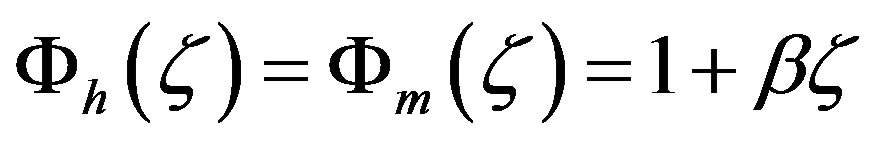 , where
  is the local stability function for sensible heat related to the nondimensional gradient of the potential temperature by
 . (2.4)
This equation is based on the similarity hypothesis  (e.g., [13]). Here,
  is the temperature scale that serves to compute
  according to
 (2.5)
(2.5)
Since  is also considered as invariant with height, water substances must not undergo phase transition processes. Under such a condition, the integration of Equation over the layer
  of the ASL yields
 . (2.6)
These profile function for the mean horizontal wind speed and the mean potential temperature are only valid for .
.
A couple of years later, various authors proposed the so-called KEYPS formula1 for the local similarity function for momentum given by
 . (2.7)
The KEYPS formula with  has experimentally been deduced by Businger et al. [27] for the stability range
 ; Panofsky and Dutton [28], however, recommended:
 . Formula (2.7) indicates a
  behavior for
  as expected for free convective conditions.
Apparently, such a local similarity function demands a more general solution of Equation (1.3). Panofsky [1] found it by rearranging Equation (1.3) as follows:
 . (2.8)
Integrating this equation over the layer  of the ASL yields:
 , (2.9)
where HAP’s integral similarity function for momentum is given by
 . (2.10)
Choosing  provides Equations (1.1) and (1.2). As mentioned before, this equation set is the general solution that is independent of the shape of the local similarity function and the range of thermal stratification.
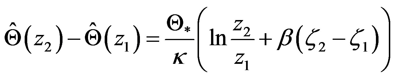
For the vertical profiles of the mean potential temperature and the mean specific humidity we obtain in a similar manner
 (2.11)
and
 , (2.12)
respectively. Here,
 (2.13)
are the integral similarity functions for sensible heat (subscript h) and water vapor (subscript q), respectively. Furthermore,  is the humidity scale related to the vertical component of the water vapor flux,
  , by
, by
 , (2.14)
and  is the local similarity function for water vapor related to the non-dimensional gradient of the specific humidity by
 . (2.15)
This equation is based on the similarity function  (e.g., [13]). When the transfer of water vapor across the ASL plays a notable role like over water surfaces and wet soil or vegetation, it is indispensable to use the following expression for the Obukhov stability length [29]:
 , (2.16)
where  is the specific heat at constant pressure for dry air. Note that long-lived trace gases can be handled in a similar manner, where it is often assumed that the local similarity function for such trace gases,
  , is equal to that of water vapor.
As discussed by various authors [13,18,30], the local similarity functions,  ,
,  , and
, and , impose as universal laws for describing the surface (constant flux) layer turbulence. Reviews of field campaigns and empirical findings can be found in [26,31-36].
3. Integral Similarity Functions for Unstable Stratification
Even though the O’KEYPS formula was established for covering the entire unstable range from close to neutral stratification to free convective conditions, another local similarity function for unstable stratification was eventually proposed by Businger [37], Dyer (unpublished; see [38]), and Pandolfo [39]. It reads
 , (3.1)
where  is another empirical constant. This equation is called the Businger-Dyer-Pandolfo relationship. It has experimentally been proved by Dyer and Hicks [41], Businger et al. [27] and others, where their results mainly covered the stability range
  (e.g., [28,33,35, 36,40], and Figure 1). From a physical point of view the
O’KEYPS formula seems to be more preferable than the Businger-Dyer-Pandolfo relationship because the O’ KEYPS formula can be related to the local balance equation of the turbulent kinetic energy if the conditions of stationary state and horizontal homogeneity are fulfilled (e.g., [13]).
Since the O’KEYPS formula seems to be bulky, Carl et al. [45] and Gavrilov and Petrov [46] eventually proposed the expression
 (3.2)
(3.2)
for the stability range , where
  was determined using observations from various locations. This equation reflects the same asymptotic behavior like the O’KEYPS formula, but notably differs from that of the Businger-Dyer-Pandolfo relationship (see Figure 2).
Businger [37] and Pandolfo [39] also suggested the following relationship between the local similarity functions for momentum und sensible heat:
 . (3.3)
Dyer and Hicks [41] eventually proved Equation (3.3) for the stability range . Since the so-called gradient-Richardson number Ri may be expressed by the non-dimensional gradients, i.e.,
 , (3.4)
the Businger-Pandolfo relationship 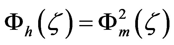 for unstable stratification provides (see Figures 3 and 4).
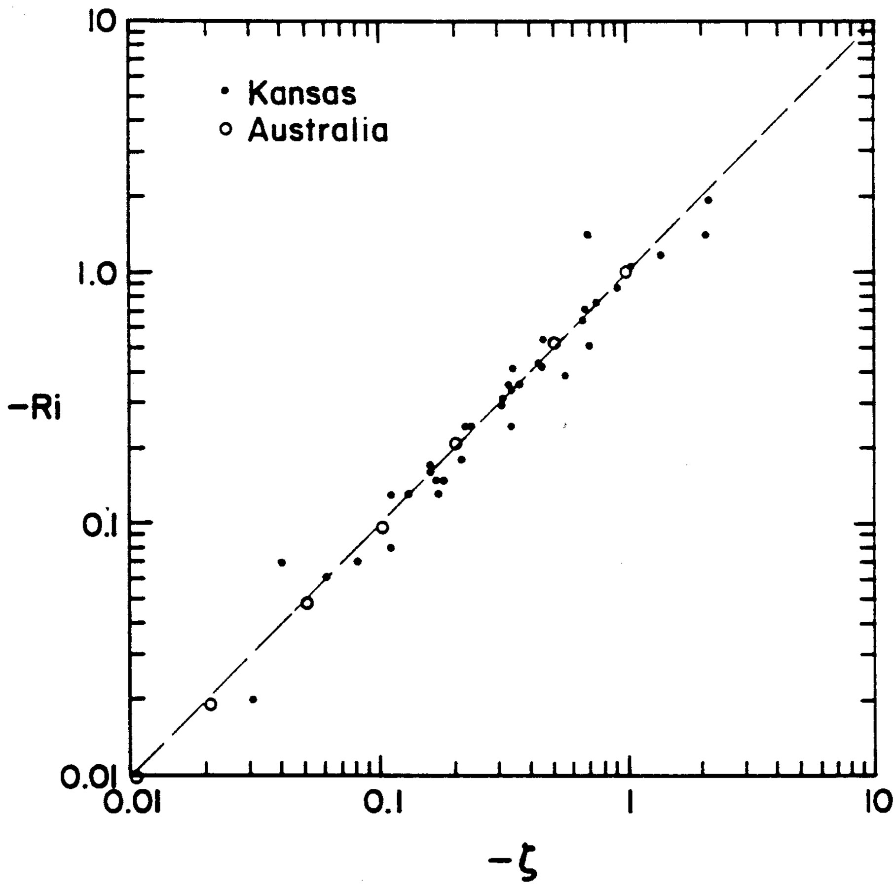
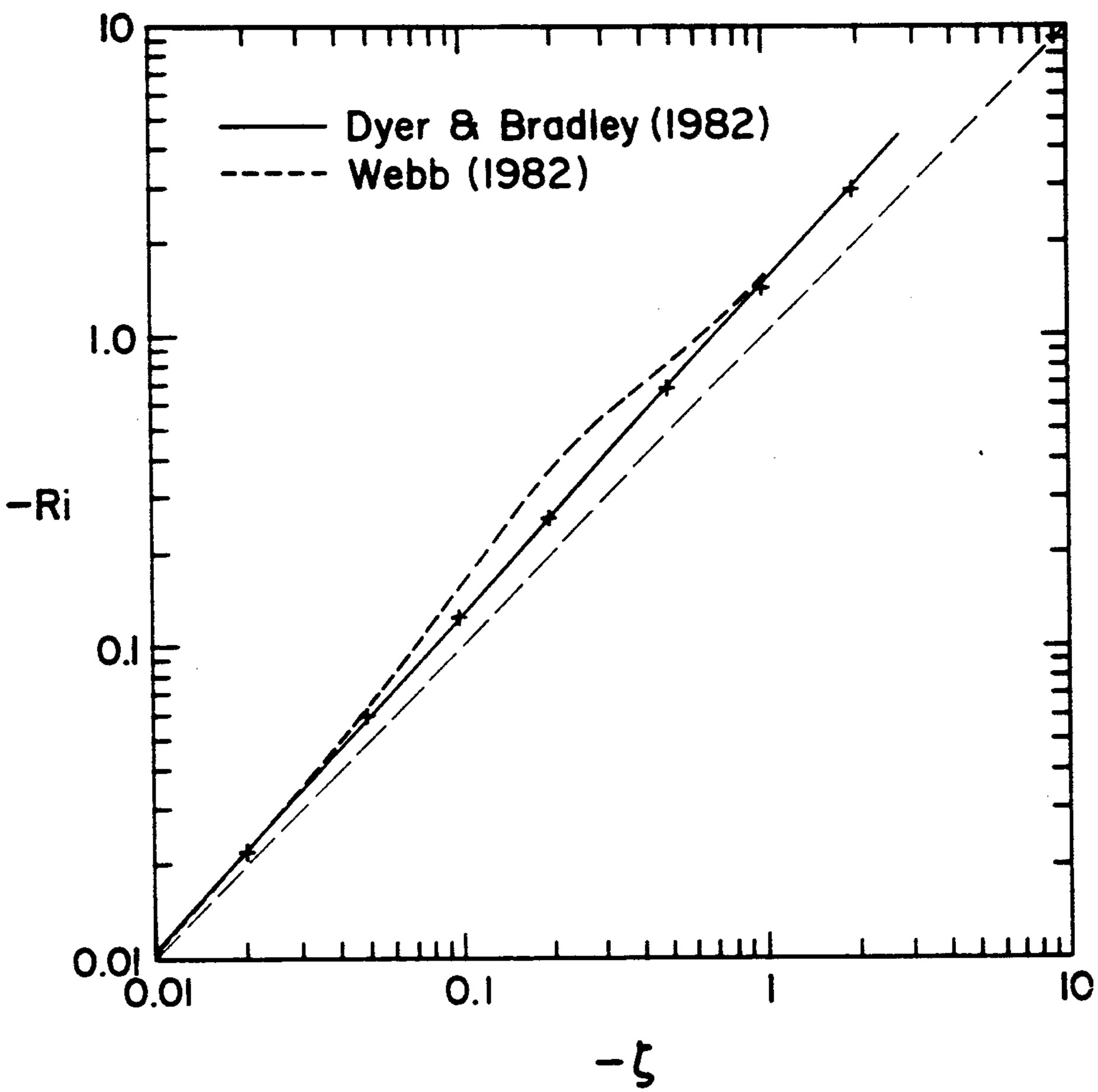
Figure 3. Gradient Richardson number, Ri, versus the Obukhov number  for three different field experiments (adopted from Businger [38]). Note that the references Dyer and Bradley (1982) and Webb (1982) are listed here as references [42,47].
 . (3.5)
However, based on the data of the 1968 Kansas field experiment [48], Businger et al. [27] suggested
 (3.6)
(3.6)
and
 (3.7)
(3.7)
for , where
  and
and  (see Figure 2). These local similarity functions provide
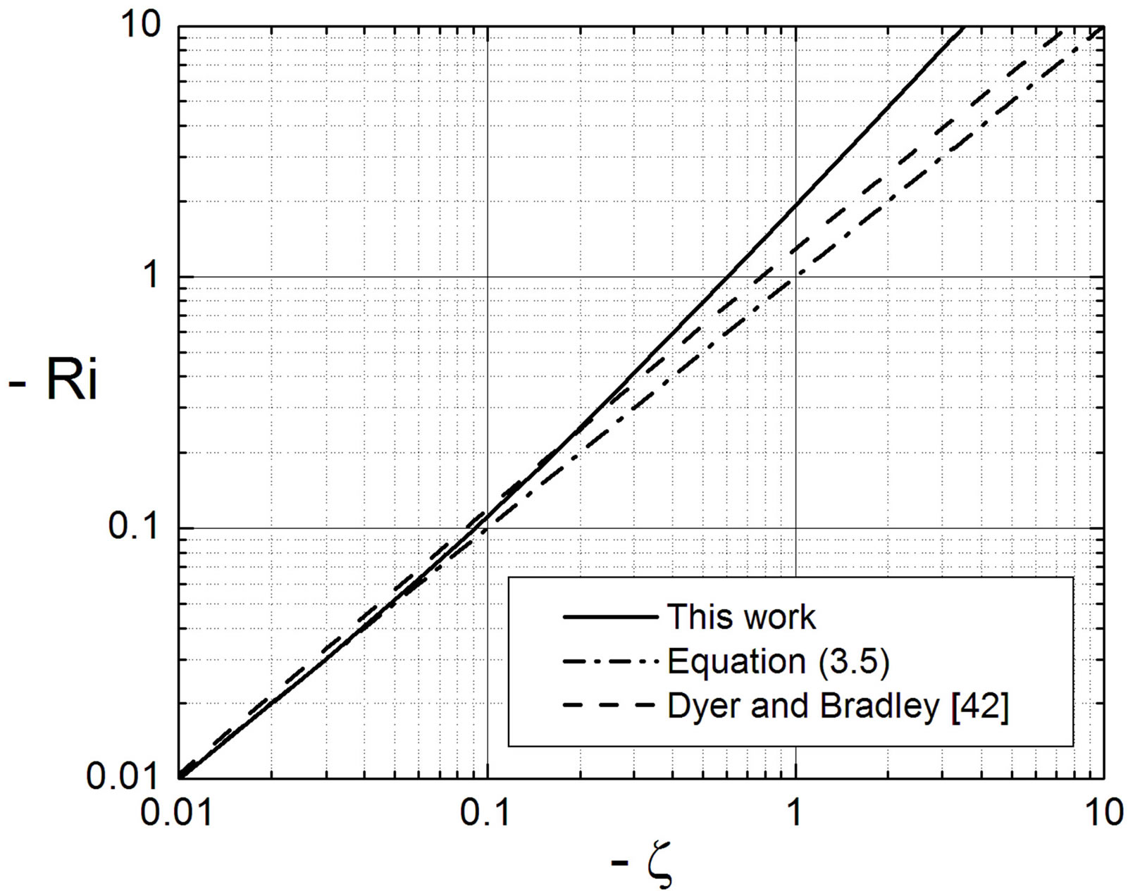
Figure 4. Gradient Richardson number, Ri, versus the Obkhov number,  , for unstable stratification, where Ri has been deduced on the basis of formulae (3.2), (3.4), and (3.26). The one-to-one line represents
  (see Equations (3.3) to (3.5)).
 . (3.8)
Consequently,  , i.e., the identity
  would be no longer valid for unstable stratification. Dyer and Bradley [42] and Webb [47] pointed out that small deviations from this identity might occur. However, as illustrated Figure 3, they found
 . Note that Högström [40] re-calibrated the local similarity functions of various authors listed in Figure 1 with respect to
 . Thus, the local similarity functions illustrated in this figure are Högström’s modified versions of
  and
and  (The same is true in case of stable stratification). A value of
  is, indeed, widely recommended. However, based on 553 independent determinations of
  (the largest, most comprehensive atmospheric data set ever used to evaluate the von Kármán constant) Andreas et al. [49] derived a value of
 , constant for
 , where
  is the roughness Reynolds number, and
  is the kinematic viscosity. Frenzen and Vogel [50] also found a value of
 , but their result is based on 29 data pairs only. Nevertheless, we do not recommend a recalibration of the local similarity functions with respect to a certain value of the von Karmán constant. Instead,
  and
and  should be used with the original values of
 . Using, for instance, the original ones of Businger et al. [27] and a von Kármán constant of
  is a notable source of inconsistency.
At the end of the sixties, the time was ripe for determining Panofsky’s integral similarity function on the basis of empirically determined local similarity functions. Paulson [19] was the first who derived integral similarity functions for unstable stratification represented here in the more general form for the layer  of the ASL:
O’KEYPS formula:
 (3.9)
(3.9)
Businger-Dyer-Pandolfo relationship:
 (3.10)
and
 , (3.11)
where
 (3.12)
are the reciprocal expressions of the local similarity functions for momentum at the two heights  and
and .
.
Obviously, the O’KEYPS solution (3.9) seems to be more bulky than that obtained with the Businger-DyerPandolfo relationship given by Equation (3.10). This might be the reason why the latter has been more widely used, even though the former has a stronger physical background [13].
Since Paulson [19] assumed that  and, hence,
  , his solutions substantially agree with Equations (3.9) to (3.11), i.e.,
 (3.13)
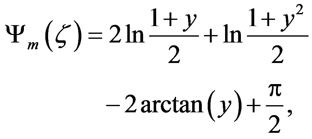 (3.14)
and
 , (3.15)
where  and the identity
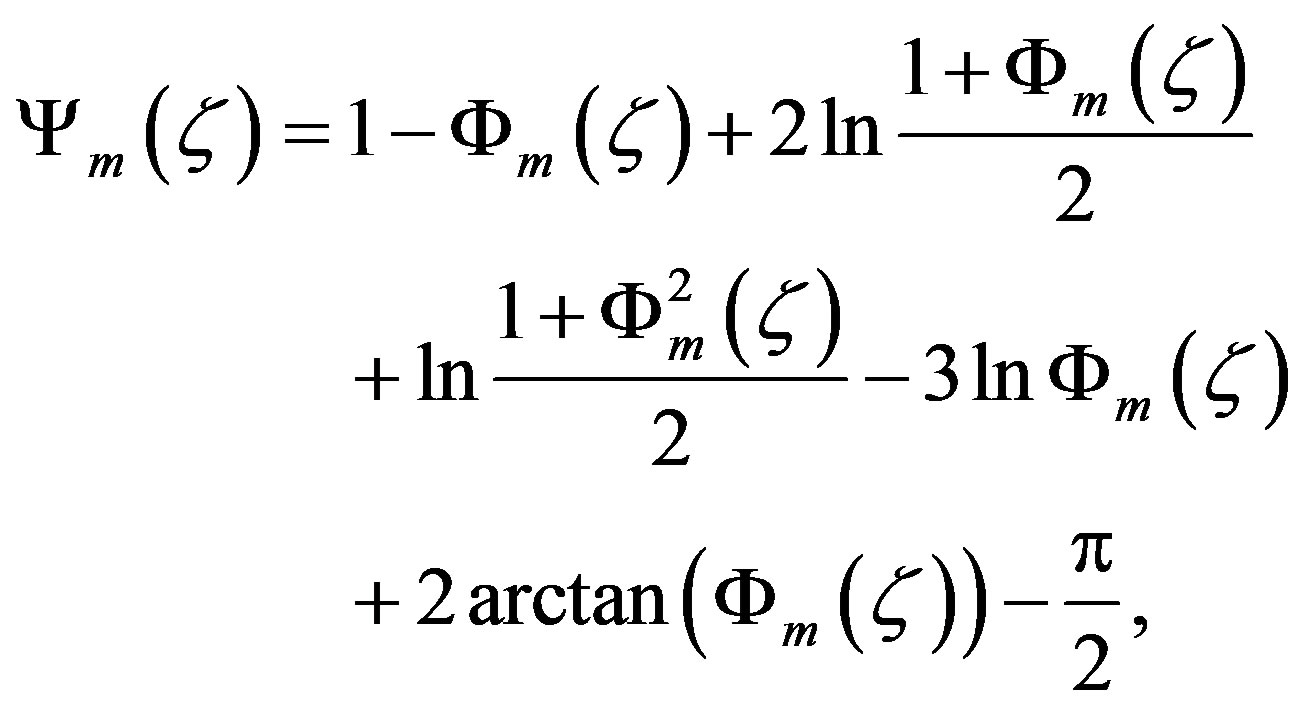
with  have been used. Often, HAP’s integral similarity function is written as
 where Paulson’s Equations (3.13) to (3.15) are considered for both
  and
and . This kind of splitting is highly awkward because it is neither reasonable nor advantageous. In addition, Paulson derived his equations for
 . Thus, the quantity
  is always equal to zero if Paulson’s Equation (3.13) to (3.15) are considered [51].
Lettau [52] eventually presented the solution for the local similarity function of Carl et al. [45] (see Equation (3.2)). It reads in the more general form for the layer  of the ASL:
 , (3.16)
where
 (3.17)
are the reciprocal expressions of the local similarity functions for momentum at the two heights  and
and , and
, and
 . (3.18)
Lettau’s [52] solution substantially agrees with Equations (3.16) to (3.18) for  and, hence,
  is considered. The integral similarity functions for momentum, (3.9), (3.10), and (3.16) are illustrated in Figure 5. As expected, formulae (3.9) and (3.16) only differ hardly when
  tends to Obukhov numbers much smaller than zero, i.e.,
  , representing freeconvective conditions. Simultaneously, the difference between Equation (3.10) and the other two formulae grows continuously. Thus, we recommend to use the integral similarity function (3.16) for practical purposes. Its results are close to those provided by the O’KEYPS solution, but the former is more convenient than the latter.
Under the assumption that the Businger-Pandolfo relationship  holds for the entire range of unstable stratification and that the local similarity function for momentum is given by Equation (3.2) we obtain
 . (3.19)
This local similarity function illustrated in Figure 2
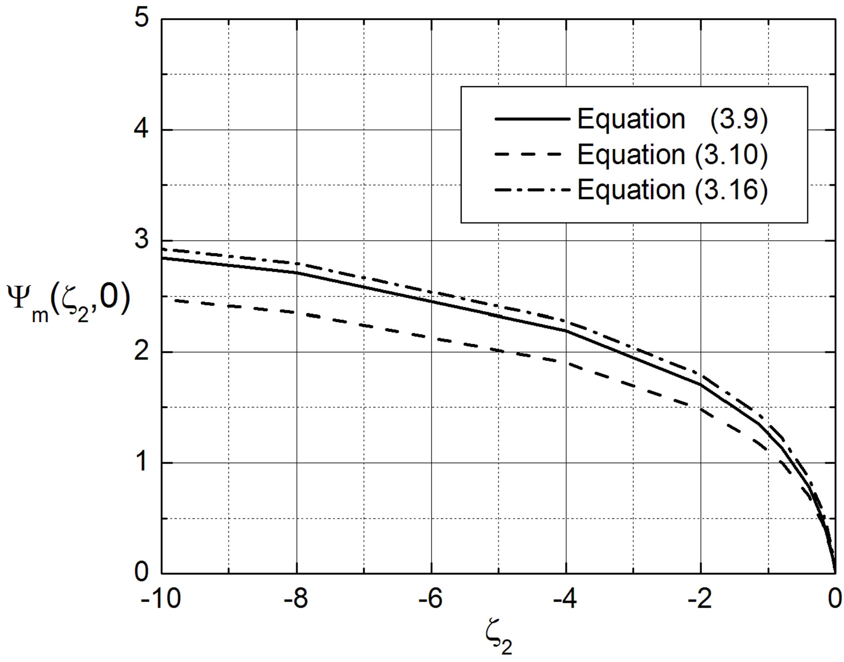
Figure 5. The integral similarity function for momentum,  , provided by formulae (3.9), (3.10), and (3.16) and plotted against the Obukhov number
 .
.
leads to [13]
 (3.20)
where  and
and  are given by Equations (3.17) and (3.18), respectively.
In the case of free convective conditions, i.e.,  , scaling owing to Prandtl [53], Obukhov [54], and Priestley [55] is considered. It is based on the similarity hypothesis
  leading to
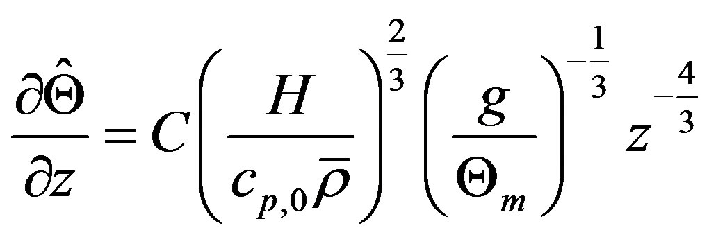 , (3.21)
where  is Priestley’s constant (e.g., [13,34]). The negative sign is required to guarantee a lapse rate in case of free convective conditions for which
  is considered. In accord with the definition of the Obukhov number (see Equation (2.16)), the free convective condition
  means that the friction velocity is of minor importance (e.g., [2,56]). It may be expressed by [2]
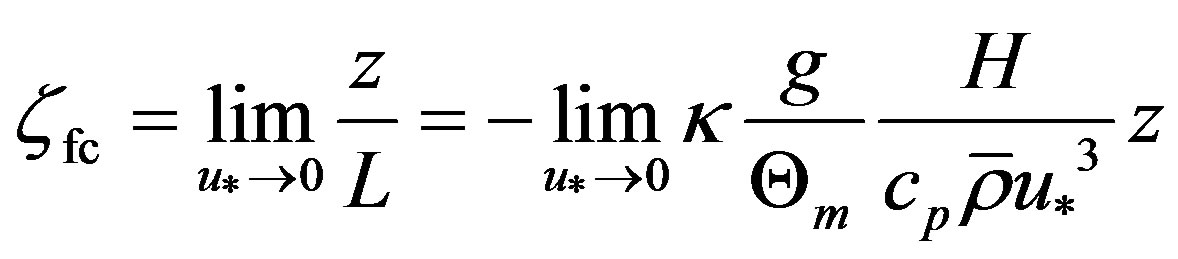 , (3.22)
where the subscript “fc” indicates free convective conditions.
Integrating Equation (3.21) over the layer  of the ASL leads to the Priestley-Estoque relation (e.g., [13, 57])
 (3.23)
with
 , (3.24)
where . For
. For  one obtains the solution of Monin and Obukhov [2] presented by their Equation (61).
Priestley’s constant was recently re-estimated by Dillon Amaya on the basis of data sets taken from the Hydrology-Atmosphere Pilot Experiment (HAPEX) in the Sahel of Niger, Africa. This field campaign was active from 1990-1992, but for the purpose of his re-estimation only data from September of 1992 were used. The corresponding data files were downloaded from the campaign’s website (www.cesbio.ups-tlse.fr/hapex, retrieved 7/2/2012). The measurements were carried out over areas of degraded fallow bush, which had once been an agricultural center, but has been left to naturally restore its fertilization. Amaya found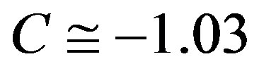 , i.e., this value is, on average, 4% smaller than the commonly accepted value (for more details, see [58]).
Rearranging Equation (3.21) in the sense of MoninObukhov scaling, where only dry air is considered (i.e., the influence of water vapor is ignored), leads to (e.g., [2,13,34,59])
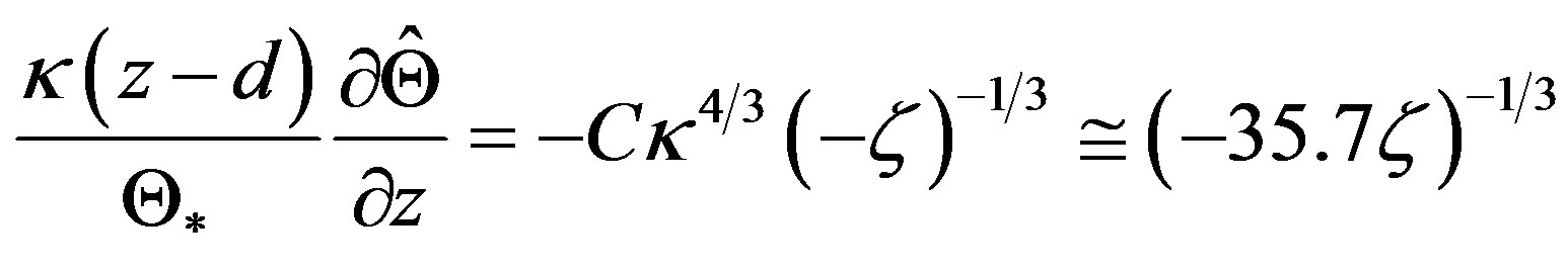 (3.25)
if Amaya’s value for the Priestley constant and a von Karman constant of  are assumed. For comparison: Based on the Cimljansk experiment, Zilitinkevič and Čalikov [43] found
 , but only for the stability range
 . Note that the local similarity functions for sensible heat given either by Equation (3.3) or Equation (3.7), commonly used, do not converge to the asymptotic solution (3.25) for
  (see Figure 2). The same is true in case of Equation (3.19). This means that the Businger-Pandolfo relationship
  is not valid for the entire range of unstable stratification. To avoid this weakness, we suggest the following local similarity function for sensible heat [58]:
 (3.26)
with . It is illustrated in the lower part of Figure 1 together with those deduced from various past field campaigns. Obviously, this local similarity function is in substantial agreement with Högström’s [40] field data for the stability range
  and tends to the free convective conditions as described by Prandtl-ObukhovPriestley scaling (see Figure 2). The gradient Richardson number deduced on the basis of Equations (3.2), (3.4), and (3.26) is illustrated in Figure 4. As suggested by Dyer and Bradley [42] and Webb [47], the condition
  is fulfilled, but the deviation from the one-toone line characterized by
  is notably stronger than empirically found, for instance, by Dyer and Bradley [42].
Equation (3.26) can be handled like Equation (3.2). Thus, one obtains:
 (3.27)
 , (3.28)
and
 . (3.29)
The integral similarity functions given by Formulae (3.11), (3.20), and (3.27) are illustrated in Figure 6. Obviously, the difference between the formulae (3.11) and (3.27) is small, but both differ notably from that given by Equation (3.20).
4. Integral Similarity Functions for Stable Stratification
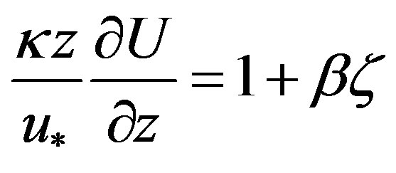
As mentioned before, Monin and Obukhov [2] already proposed for stable stratification (and weakly unstable stratification) a linear relationship of the form
 (4.1)
(4.1)
later experimentally proved by Čalikov [60], Zilitinkevič

Figure 6. The integral similarity function for sensible heat,  , provided by formulae (3.11), (3.20), and (3.27) and plotted against the Obukhov number
 .
.
and Čalikov [43], Businger et al. [27] and others mainly for the stability range , but there is a large scatter in the case of momentum with some values of
  for
for  (see Figures 7 and 8). Dyer [31] and Panofsky and Dutton [28] recommended a value of
  which is close to that of Webb [61]. This value is much larger than
  mentioned before (see Equation (2.1)).
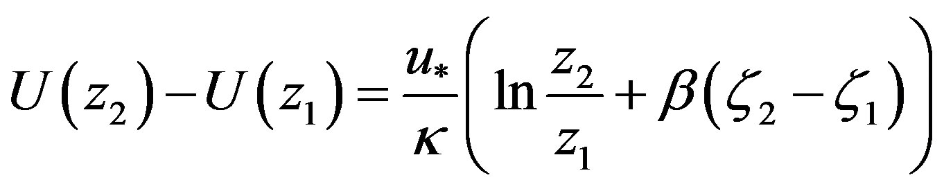
The integration of Formula (4.1) over the layer  of the ASL provides for the integral similarity function
 . (4.2)
This integral similarity function leads to a similar form as already suggested by Monin and Obukhov [2], even though the parameters  and
and  differ considerably. As aforementioned, Monin and Obukhov [2] also proposed the relationship
 , (4.3)
also recommended by Webb [61]. In accord with Equation , this relationship provides
 (4.4)
(4.4)
or
 . (4.5)
Based on the 1968 Kansas field experiment [48], Businger et al. [27], however, suggested for stable stratification:
 (4.6)
(4.6)
and
 (4.7)
(4.7)
with  (see Figures 7 and 8).
The integration of these formulae over the layer  of the ASL yields
 (4.8)
(4.8)
and
 . (4.9)
As expected, the integral similarity functions (4.2) and (4.8) are nearly identical (see Figure 9). They only differby the parameters  and
and . In contrast to this behavior, the Formula (4.9) notably differs from both other equations, where, in addition,
  must fulfill the condi-
tion . Compared with Equation (2.11), it provides a notably different profile function
 . (4.10)
Inserting the local similarity functions (4.6) and (4.7) into Equation (3.4) provides
 . (4.11)
Obviously, for stable stratification the influence of the term  weakens gradually as
  increases, i.e., as illustrated in Figure 10, the results inferred from Formulae (4.4) and (4.11) only differ slightly for strongly stable stratification. This small difference is mainly related to the parameters
  and
and .
.
Two prominent difficulties can be attributed to the use of these parameterization principles:
Since  is commonly recommended, the gradient Richardson number has to satisfy the condition
  because Equation (4.5) would become indeterminate for
 , and
, and  would be negative for
 . The latter contradicts the definition of stable stratification for which
  [62]. Rearranging Equation (4.11) leads to
 (4.12)
Thus, the condition  has to be fulfilled to prevent that
  becomes negative if
  is used. This means that in these two cases the gradient Richardson number is always notably lower than the critical Richardson number customarily assumed to be
 (e.g., [13,28]), even though Ellison [63] found gradient Richardson numbers up to
  in wind tunnel experiments.
According to Högström [40] and Cheng and Brutsaert [64], reliable values of the Obukhov number satisfy the condition  when stable stratification prevails. This means that for
  the gradient Richardson number amounts to
  in case of Equation (4.4) and to
  in case of Equation (4.11). As the gradient Richardson number and the flux Richardson number,
  , are related to each other by
  and the turbulent Prandtl number is given by
  , the assumption
  [2,61] would lead to
 , and, hence, to
 . This means that under such condition the flux Richardson number would be restricted according to
  . This value is much smaller than the value of
  that characterizes the fact that mechanical gain of TKE equals the thermal loss of TKE so that the turbulent flow becomes increasingly viscous (laminar) due to the dissipation of energy [13]. As discussed by Mölders and Kramm [62], the restriction of
  was Louis’ [65] reason to introduce a parametric model with which he artificially enhanced the transfer coefficient for sensible heat for strongly stable stratification to prevent “that once the bulk Richardson number (derived from
  using finite differences) exceeds its critical value, the ground becomes energetically disconnected from the atmosphere and starts cooling by radiation at a faster rate than is actually observed”.
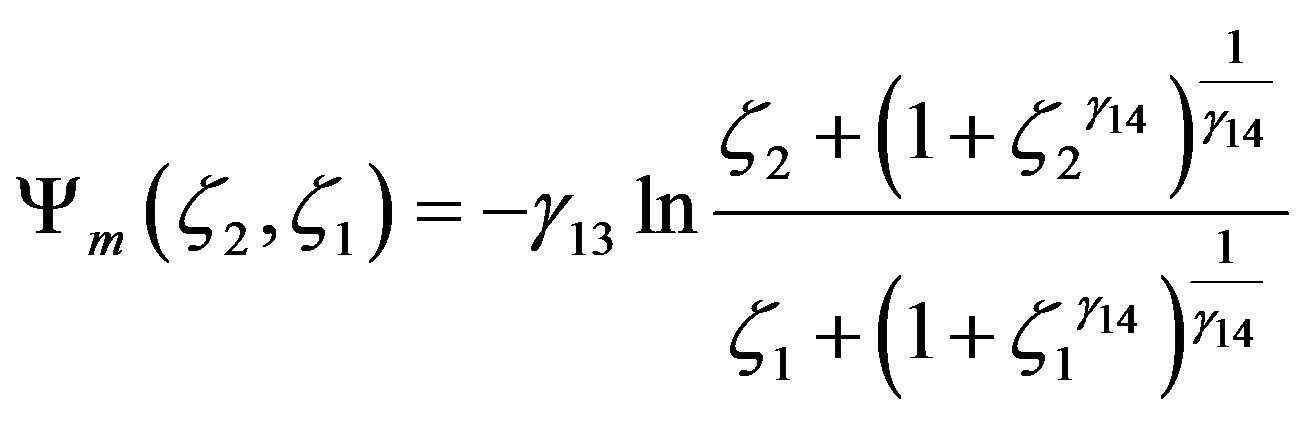
To prevent such an energetic disconnection Beljaars and Holtslag [66] first discussed the following integral similarity functions for momentum and sensible heat that is based on the work of Holtslag and De Bruin [67]:
 (4.13)
and , where
 ,
,  ,
,  , and
, and . Here, this formula is presented for the layer
  of the ASL. For
  one immediately obtains their original one (see Figure 9). Since
 , (4.14)
the corresponding local similarity function reads [62]:
 . (4.15)
As illustrated in Figure 8, this formula notably differs from Webb’s [61] recommendation. The corresponding gradient Richardson number determined on the basis of Equation (3.4) is also shown in Figure 10. Obviously, these local similarity functions for momentum and sensible heat result in a gradient Richardson number up to  for
for , i.e., it is already larger than
 . If
. If  increases the
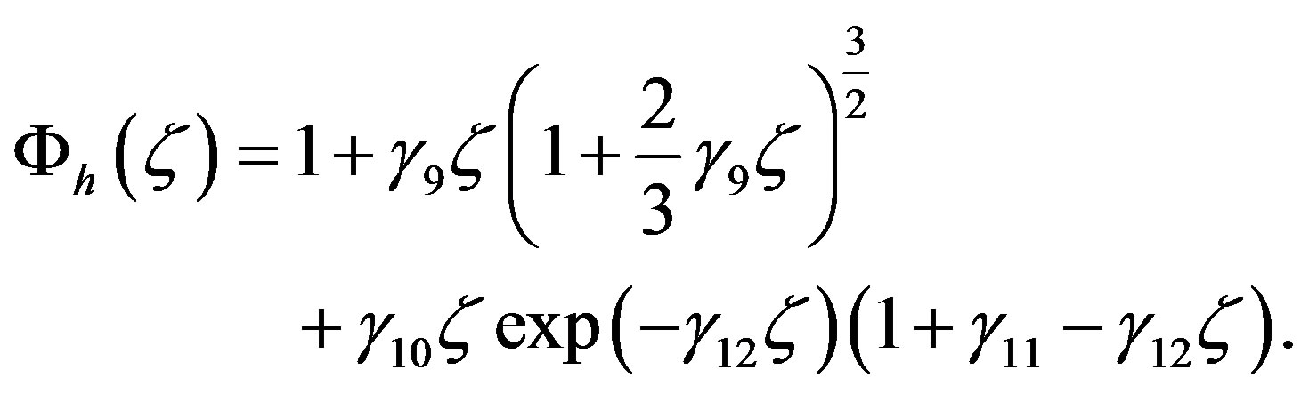
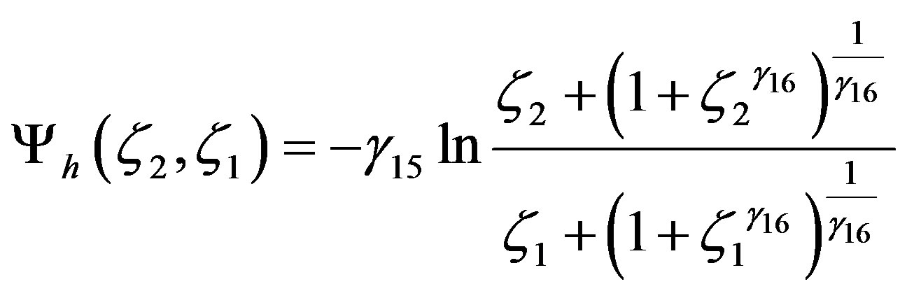
  value will also increase. To obtain results more consistent with critical Richardson number considerations Beljaars and Holtslag [66] proposed for the integral similarity function for sensible heat:
 (4.16)
again presented here for the layer  of the ASL. The corresponding the local similarity function reads:
 (4.17)
Beljaars and Holtslag [66] recommended ,
,  ,
,  , and
, and  for both, Equation (4.13) and Equation (4.16). This change has the effect that the gradient Richardson number increases up to
  for
for , i.e., it is still larger than
 . Again, if
  increases the
  value will increase rapidly.
Recently, Cheng and Brutsaert [64] suggested for the entire range of stable stratification  following formulae:
 (4.18)
and
 , (4.19)
where ,
,  ,
,  , and
, and . For neutral conditions, i.e.,
  , one obtains
 . For moderately stable stratification both formulae can be approximated by linear expressions, i.e.,
  and
and , but for increasing stability formulae and tend to
  and
and  (see Figure 8). Obviously, for the entire range of stable stratification
  and
and  differ from each other. In contrast to the functions
  and
and  of Beljaars and Holtslag [66], which have points of inflection, the formulae of Cheng and Brutsaert [64] are bounded [62]. The relationship between the gradient Richardson number and the Obukhov number is also illustrated in Figure 10. Obviously, gradient Richardson numbers up to
  occur for
 . As in case of the local similarity functions of Beljaars and Holtslag [66], if
  increases the
  value will also increase. Since the local similarity functions of Cheng and Brutsaert [64] are bounded, this increase of
  is finally proportional to
 .
.
The results for strongly stable stratification have been considered with care. As reported by Cheng and Brutsaert [64], the calculated  data points for
  were excluded from their analysis because the larger scatter suggested either unacceptable error in the measurements or perhaps other unexplained physical effects. According to them, a possible reason could be that these data points are already outside the stable surface layer so that Monin-Obukhov similarity for the transfer of momentum und sensible heat across the ASL may not further be valid [13].
The Formulae (4.18) and (4.19) provide logarithmic profiles for neutral and strongly stable stratification. The latter, already found by Webb [61] and Handorf et al. [68], seems to be awkward because if the magnitude of turbulent fluctuations decreases towards the small values of the quiet regime with increasing stability (e.g. [69,70]), the near-surface flow should become mainly laminar. For a pure laminar flow, viscous effects dominate leading to ,
,  , and
, and , where
  and
and  are the Prandtl number and the Schmidt number for water vapor, respectively. Thus, linear profiles have to be expected [13]. The same is true when the respective eddy diffusivities become invariant with height. Such height invariance might be possible when the quiet regime prevails and the magnitude of the turbulent fluctuations is small across the entire ASL. Thus, we have to assume that Monin-Obukhov similarity is incomplete under strongly stable conditions. If under such conditions the constant flux approximation is no longer valid as debated, for instance, by Webb [61] and Poulos and Burns [71], Monin-Obukhov similarity must not be expected [13,62].
The solutions for the local similarity functions  and
and  given by Formulae (4.18) and (4.19) for the layer
  of the ASL read:
 (4.20)
and
 . (4.21)
For , one obtains the original expressions of Cheng and Brutsaert [64]. These integral similarity functions are illustrated in Figure 9, together with those related to Webb [61], Businger et al. [27], and Beljaars and Holtslag [66].
5. Final Remarks and Conclusions
With his new profile function for the mean, horizontal wind speed and his integral similarity function for momentum HAP opened the door for Monin-Obukhov scaling in a wide range of micrometeorological and microclimatological applications. All empirical and semitheoretical expressions for the local similarity functions ,
,  , and
, and  that can be found in the literature may be inserted in his concept of the integral similarity function, even though numerical integration might be required. Fortunately, in most cases the integration can be performed elementarily. For the aforementioned applications, we currently recommend Equations (3.2) and (3.26) for unstable stratification
 , leading to the integral similarity functions (3.16) and (3.27), and Equations (4.18) and (4.19) for stable stratification
 , leading to the integral similarity functions (4.20) and (4.21).
As there are some indications that Monin-Obukhov similarity is no longer valid in case of strongly stable stratification  probably owing to incomplete similarity, further research should focus on this range of diabatic stratification.
6. Acknowledgements
We would like to express much gratitude to the National Science Foundation for funding Dillon Amaya’s project work in summer 2012 through the Research Experience for Undergraduates (REU) Program, grant AGS1005265. We would like to extend gratitude to the scientists of the HAPEX field campaign, specifically Drs. Lutz Lech, Heiner Billing, Hans-Jürgen Bolle, Matthias Eckardt, and Ines Langer, for compiling a very accessible data set.
NOTES
1KEYPS stands for the initials of various authors who proposed this formula (Kazansky and Monin [20], Ellison [21], Yamamoto [22], Panofsky [23], and Sellers [24]). As Obukhov already suggested it in 1946, the KEYPS formula was eventually renamed in O’KEYPS formula (e.g., [13,25,26]).