1. Introduction
Based on observations [1-3], we can say that the universe today is almost flat. If this is the case, i.e., it has remained flat since the beginning of time? To this problem of flatness, we can add the horizon problem. To solve these problems Englert and Guth proposed in [1] primordial inflation. The universe would have grown exponentially just after the Big Bang. Many models of inflation exist and most involve a scalar field which undergoes a phase transition during inflation. Many of these models use a potential that needs to be adjusted so that the theory is consistent with the observations. In this paper, we develop models of inflation from non minimal coupling to gravity. The first scalar-tensor theories involving nonminimal couplings are known as coupling Brans-Dike [4]. This work is based on an article published in 1974 by [5] followed by [6] where they show that only four families of terms lead to a violation of the equivalence principle, while ensuring to obtain the equations of motion of the second member. These couplings are given in [6] as the “Fab Four”. In our work, we consider a Lagrangian with two parts: the first is the non-minimal derivative coupling of the form
 (1)
(1)
nicknamed John in Fab Four. The second part consists of a minimal coupling with a multiplicative potential [7]. In other words, we relied on the work of [4,8,9], but here we have a potential which multiplies the kinetic part of the Lagrangian.
After building the action, we deduced the different equations by considering a flat space. We then presented some cosmological models and which followed by a discussion of those models.
2. Mathematical Model
2.1. Action
Let  be the reduced Planck mass.
Let ,
, 
and
 (2)
(2)
Which is equivalent to
 (3)
(3)
where ε and γ are constants dimensionless coupling; κ is 1/L2,  is 1/L. This action can be written
 (4)
(4)
ε = 0, we find the models studied by [8] and [4]
2.2. Equations of Motion
Consider a spatially-flat cosmological model with the metric
 (5)
(5)
With  the scale factor and
  the Euclidian metric. If one assume
 , then the cosmological equations which derive from the action (4) can be written
 (6)
(6)
 (7)
(7)
 (8)
(8)
where

The Equations (6) and (7) are the equation of movement; 8 is the Klein-Gordon equation. If one poses

where  and
and  are respectively the pressure and the matter density of the field. We can use 6 and 7 to determine equation of state (EoS)
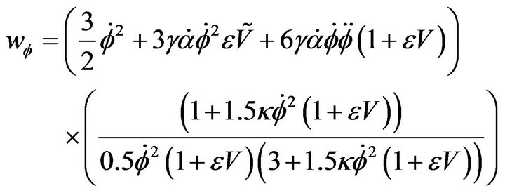 (9)
(9)
3. Results and Discussion
Given the complexity of the equations, we did not obtain solutions analytics.
3.1. Decoupled Equations
Before starting the numerical solution, we will work Equations (7) and (8) to separate  and
and 
 (10)
(10)
 (11)
(11)
We perform numerical integration by using matlab ode 45 precisely embedded Runge-Kutta method.

When , the evolution of the state equation shows that with the presence of this potential, the field acts like the dark matter for ε negative or positive. The acceleration parameter goes to zero. The field ϕ vs the scale factor is a constant. This model does not accommodate inflation. These plots (Figures 1-4) have been obtained by numerical integration for an initial condition of φ = 10 in natural units in the case γ = 1.

Here also, the field starts with an EoS  but this field likes the dark matter with state equation equal 0; the acceleration parameter is negative; the Universe only decelerates as can been shown the four following plots (Figures 5-8)

We find that we can have cosmological models for only λ negative. We have shown the curves for . compared with those obtained for
  which is studied in the model [8]. The acceleration parameter (Figure 9) shows a universe initially accelerated after some time. So this time could correspond to the end of the inflationary epoch. Note that here, when ε is negative, universe deceleration makes less pronounced. Observing the curves α(t).

Figure 1. Evolution of α(t) for ε = −1, ε = 0 and ε = 1. As shown in the graph, when ε ≠ 0, α decreases quickly.
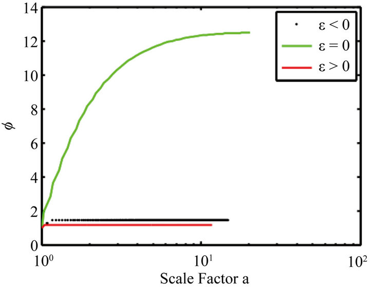
Figure 2. Evolution of the field Φ vs. the scale factor for ε = −1, ε = 0 and ε = 1. ε ≠ 0, ϕ is a constant.

Figure 3. Evolution of the EoS wϕ vs. the scale factor (which is denoted by res.a) for ε = −1, ε = 0 and ε = 1. When ε = 0, the EoS wϕ starts at −1 and evolves by oscillation to 0. But when ε = 1, wϕ jumps vertically from −1 to 0 and no longer varies.

Figure 4. Evolution of the acceleration parameter q vs. the scale factor; ε = 0, this parameter remained positive long before the descent to 0. Against by ε ≠ 0, it drops abruptly to 0 and keeps this value.

Figure 5. Evolution of α(t) for ε = 0 and ε = 1.
Figure 10 shows that these curves are linear at the origin, and this reinforces the notion of inflation at the origin of time. During this time the field  is an exponential function of the scale factor (Figure 11). During the inflationary epoch field behaved like a dark energy before undergoing a transition to the matter.