The Continuous Wavelet Transform Associated with a Dunkl Type Operator on the Real Line ()
1. Introduction
In this paper we consider the first-order singular differential-difference operator on R

where  and q is a
  real-valued odd function on R. For q = 0, we regain the differential-difference operator

which is referred to as the Dunkl operator with parameter  associated with the reflection group Z2 on R. Those operators were introduced and studied by Dunkl [1-3] in connection with a generalization of the classical theory of spherical harmonics. Besides its mathematical interest, the Dunkl operator has quantum-mechanical applications; it is naturally involved in the study of onedimensional harmonic oscillators governed by Wigner’s commutation rules [4-6].
Put
 (1)
(1)
and
 (2)
(2)
The authors [7] have proved that the integral transform
 (3)
(3)
is the only automorphism of the space  of
of  functions on R, satisfying

for all  The intertwining operator X has been exploited to initiate a quite new commutative harmonic analysis on the real line related to the differential-difference operator Λ in which several analytic structures on R were generalized. A summary of this harmonic analysis is provided in Section 2. Through this paper, the classical theory of wavelets on R is extended to the differential-difference operator Λ. More explicitly, we call generalized wavelet each function g in
  satisfying almost all

where  denotes the generalized Fourier transform related to Λ given by

 being the solution of the differential-difference equation

Starting from a single generalized wavelet g we construct by dilation and translation a family of generalized wavelets by putting

where  stand for the generalized dual translation operators tied to the differential-difference operator Λ, and ga is the dilated function of g given by the relation

Accordingly, the generalized continuous wavelet transform associated with Λ is defined for regular functions f on R by

In Section 3, we exhibit a relationship between the generalized and Dunkl continuous wavelet transforms. Such a relationship allows us to establish for the generalized continuous wavelet transform a Plancherel formula, a point wise reconstruction formula and a Calderon reproducing formula. Finally, we exploit the intertwining operator X to express the generalized continuous wavelet transform in terms of the classical one. As a consequence, we derive new inversion formulas for dual operator  of X.
of X.
In the classical setting, the notion of wavelets was first introduced by J. Morlet, a French petroleum engineer at ELF-Aquitaine, in connection with his study of seismic traces. The mathematical foundations were given by A. Grossmann and J. Morlet in [8]. The harmonic analyst Y. Meyer and many other mathematicians became aware of this theory and they recognized many classical results inside it (see [9-11]). Classical wavelets have wide applications, ranging from signal analysis in geophysics and acoustics to quantum theory and pure mathematics (see [12-14] and the references therein).
2. Preliminaries
Notation. We denote by
•  the class of measurable functions f on R for which
  where
where

and 
•  the class of measurable functions f on R for which
  where Q is given by (2).
•  the class of measurable functions f on R for which
Remark 1. Clearly the map
 (4)
(4)
is an isometry
• from  onto
onto ;
;
• from  onto
onto .
.
2.1. Generalized Fourier Transform
The following statement is proved in [7].
Lemma 1. 1) For each , the differential-difference equation

admits a unique  solution on R, denoted
 , given by
 (5)
(5)
where  denotes the one-dimensional Dunkl kernel defined by

 being the normalized spherical Bessel function of index
  given by

2) For all ,
,  and
and  we have
 (6)
(6)
3) For each  and
and , we have the Laplace type integral representation
 (7)
(7)
where  is given by (1).
The generalized Fourier transform of a function f in  is defined by
 (8)
(8)
Remark 2. 1) By (6) and (7), it follows that the generalized Fourier transform  maps continuously and injectively
  into the space
  of continuous functions on R vanishing at infinity.
2) Recall that the one-dimensional Dunkl transform is defined for a function  by
by
 (9)
(9)
Notice by (5), (8) and (9) that
 (10)
(10)
where M is given by (4).
Two standard results about the generalized Fourier transform  are as follows.
Theorem 1 (inversion formula). Let  such that
 . Then for almost all
  we have

where
 (11)
(11)
Theorem 2 (Plancherel). 1) For every , we have the Plancherel formula

2) The generalized Fourier transform  extends uniquely to an isometric isomorphism from
  onto
onto .
.
2.2. Generalized Convolution
Recall that the Dunkl translation operators  are defined by
 (12)
(12)
where  is a finite signed measure on R, of total mass 1, with support

and such that . For the explicit expression of the measure
  see [15].
Define the generalized translation operators Tx,  , associated with Λ by
 (13)
(13)
By (12) and (13) observe that
 (14)
(14)
The generalized dual translation operators are given by
 (15)
(15)
We claim the following statement.
Proposition 1. 1) Let f be in 
 Then for all
 is a well defined element in
  and
and

2) Let f be in 
 Then for all
 ,
,  is well defined as a function in
  and
and

3) For  p = 1 or 2, we have

4) Let ,
,  such that
  If
If  and
and  then we have the duality relation

Proof. 1) By (14) and [13, Equation (8)] we have

2) By (15) and [13, Equation (8)] we have

3) By (5), (10), (15) and [1, Theorem 11] we have

4) By (14), (15) and [1, Theorem 11] we have

This concludes the proof. ■
The generalized convolution product of two functions f and g on R is defined by
 (16)
(16)
Remark 3. Recall that the Dunkl convolution product of two functions f and g on R is defined by
 (17)
(17)
By virtue of (15), (16) and (17) it is easily seen that
 (18)
(18)
By use of (10), (18) and the properties of the Dunkl convolution product mentioned in [16], we obtain the next statement.
Proposition 2. 1) Let  such that
 If
If  and
and  then
then
 and
and
 .
.
2) For  and
and  p = 1 or 2, we have

2.3. Intertwining Operators
According to [7], the dual of the intertwining operator X given by (3), takes the form

It was shown that  is an automorphism of the space
  of
of  compactly supported functions on R, satisfying the intertwining relation

where  is the dual operator of Λ defined by

Moreover, we have the factorizations
 (19)
(19)
where  and
and  are respectively the Dunkl intertwining operator and its dual given by


Using (19) and the properties of  and
and  provided by [17], we easily derive the next statement.
Proposition 3. 1) If  then
then 
and 
2) If  then
then  and
and

3) For every  and
and  we have the duality relation

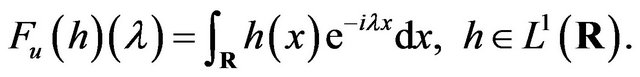
4) For every  we have the identity
 (20)
(20)
where Fu denotes the usual Fourier transform on R given by
5) Let . Then

where * denotes the usual convolution product on R given by

6) Let  and
and  Then
Then
 (21)
(21)
3. Generalized Wavelets
Notation. For a function f on R put

3.1. Dunkl Wavelets
Definition 1. A Dunkl wavelet is a function  satisfying the admissibility condition
 (22)
(22)
for almost all 
Notation. For a function g in  and for
  we write
 (23)
(23)
where  are the Dunkl translation operators given by (12), and
 (24)
(24)
Definition 2. Let  be a Dunkl wavelet. The Dunkl continuous wavelet transform is defined for smooth functions f on R by
 (25)
(25)
which can also be written in the form
 (26)
(26)
where  is the Dunkl convolution product given by (17).
The Dunkl continuous wavelet transform has been investigated in depth in [17] from which we recall the following fundamental properties.
Theorem 3. Let  be a Dunkl wavelet. Then 1) For all
  we have the Plancherel formula

2) For  such that
  we have

for almost all 
3) Assume that  For
For  and
and  the function

belongs to  and satisfies

3.2. Generalized Wavelets
Definition 3. We say that a function  is a generalized wavelet if it satisfies the admissibility condition
 (27)
(27)
for almost all 
Remark 4. 1) The admissibility condition (27) can also be written as

2) If g is real-valued we have , so (27) reduces to

3) If  is real-valued and satisfies
  such that
 , as
, as  then (27) is equivalent to
4) According to (10), (22) and (27),  is a generalized wavelet if and only if,
  is a Dunkl wavelet, and we have
 (28)
(28)
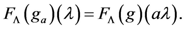
Notation. For a function g on R and , put
, put
 (29)
(29)
Remark 5. Notice by (24) and (29) that
 (30)
(30)
Proposition 4. 1) Let  and
and  for some
  Then
Then  and
and

where q is such that 
2) For  and
and  p = 1 or 2, we have
Proof. 1) By (30) and [13, Equation (13)], we have

2) By (10), (30) and [13, Equation (11)], we have

which achieves the proof. ■
Definition 4. Let  be a generalized wavelet. We define for regular functions f on R, the generalized continuous wavelet transform by
 (31)
(31)
where 

 (32)
(32)
and  are the dual generalized translation operators given by (15).
Remark 6. A combination of (15), (23) and (32) yields
 (33)
(33)
Proposition 5. Let  be a generalized wavelet. Then for all
  p = 1 or 2, we have
 (34)
(34)
where # is the generalized convolution product given by (16).
Proof. By (18), (25), (26), (30), (31) and (33), we have

which ends the proof. ■
A combination of Theorem 3 with identities (28), (33) and (34) yields the following basic results for the generalized continuous wavelet transform.
Theorem 4 (Plancherel formula). Let  be a generalized wavelet. Then for all
  we have

Theorem 5 (inversion formula). Let  be a generalized wavelet. If
  and
and  then we have

for almost all 
Theorem 6 (Calderon’s formula). Let  be a generalized wavelet such that
  Then for
  and
and  the function

belongs to  and satisfies

3.5. Inversion of the Intertwining Operator tX Using Generalized Wavelets
In order to invert tX we need the following two technical lemmas.
Lemma 2. Let  such that
 and satisfying
 (35)
(35)
as  Let
Let  Then
Then  and
and

where  is given by (11).
Proof. We have

As by (3) and (7),

we deduce that
 (36)
(36)
with

Clearly,  So it suffices, in view of (36) and Theorem 2, to prove that h belongs to
  We have

By (35) there is a positive constant k such that

From the Plancherel theorem for the usual Fourier transform, it follows that

which ends the proof. ■
Lemma 3. Let  be real-valued such that
  and satisfying
  such that
 (37)
(37)
as  Let
Let  Then
Then  is a generalized wavelet and
Proof. By using (37) and Lemma 2 we see that ,
,  is bounded and

Thus, in view of Remark 4 3), the function  satisfies the admissibility condition (27). ■
Recall that the classical continuous wavelet transform is defined for suitable functions f on R by
 (38)
(38)
where ,
,  and
and  is a classical wavelet on R, i.e., satisfying the admissibility condition
 (39)
(39)
for almost all  A more complete and detailed discussion of the properties of the classical continuous wavelet transform can be found in [10].
Remark 7. 1) According to [10], each function satisfying the conditions of Lemma 3 is a classical wavelet.
2) In view of (20), (27) and (39),  is a generalized wavelet, if and only if,
  is a classical wavelet and we have

In the next statement we exhibit a formula relating the generalized continuous wavelet transform to the classical one.
Proposition 6. Let g be as in Lemma 3. Let  Then for all
  p = 1 or 2, we have

Proof. By (34) we have

But

by virtue of (3), (24) and (29). So using (21) and (38) we find that

which gives the desired result.
Combining Theorems 5, 6 with Lemma 3 and Proposition 6 we get Theorem 7. Let g be as in Lemma 3. Let . Then we have the following inversion formulas for the integral transform
 :
:
1) If  and
and  then for almost all
  we have

2) For  and
and  the function

satisfies

4. Acknowledgements
This work was funded by the Deanship of Scientific Research at the University of Dammam under the reference 2012018.
NOTES