1. Introduction
This paper considered the solution to the second order initial value problem of the form
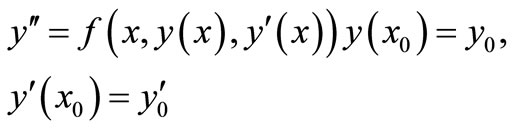 (1)
(1)
Predictor-corrector method for solving higher order ordinary differential equation has been proposed by many scholars. These authors are [1-5]. They individually proposed continuous implicit linear multistep method where separate reducing order of accuracy predictors was developed and Taylor series expansion provided the starting value. The major setback of this method is the cost of developing predictors. Moreover, the predictors developed are of lower order to the corrector; hence it has a great effect on the accuracy of the results.
In order to cater for the shortcoming of predictor-corrector method, scholars proposed block method. Block method gives solutions at each grid within the interval of integration without ovelapping and the burden of developing separate predictors is eradicated. The authors who proposed block method are [6-12]. These authors proposed a discrete block method, which did not enable evaluation at all points within the interval of integration.
In this paper, we propose a continuous block method which enables evaluation at all points within the interval of integration without starting the block all over. Continuous block method enables one to recover discrete block when evaluating at selected grid points.
2. Methodology
Given the general block formulae proposed by [11]
 (2)
(2)
where 
 is the order of the differential equation,
  is the steplenght,
  and
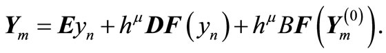
and  are matrices. We then propose a prediction equation in the form
 (3)
(3)
where  Substituting (3) into (2) gives
 (4)
(4)
Equation (4) is non self starting since the prediction equation is not gotten directly from the block formulae as proposed by [13].
In formulating the continuous block method we now consider a continuous implicit linear multistep method given by
 (5)
(5)
where  and
and  are the numbers of interpolation and collocation points.
  and
and  are polynomials.
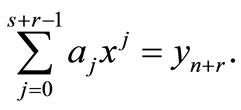
Solving (5) for the independent solution gives a continuous block formulae in the form
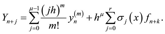 (6)
(6)
where  is a polynomial,
  Evaluating (6) at selected value of
  reduces to (2).
Development of the Continuous Block Formula
Consider power series of a single variable as our approximate solution in the form
 (7)
(7)
The second derivatives of (7) gives
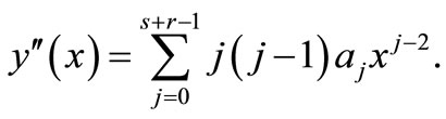 (8)
(8)
putting (8) into (1) gives
 (9)
(9)
Let the solution to (1) be soughted on the partition  with a constant stepsize
  given as

Interpolating (7) at  and collocating (9) at
  gives
gives
 (10)
(10)
 (11)
(11)
solving (10) and (11) for  and substituting back in (7) gives a continuous linear multistep method of the form
 (12)
(12)
where the coefficient of  and
and  are given as


where

Solving for the independent solution  in (13) gives a continuous block formulae (12) where the coefficient of
  is given by


Evaluating the continuous block method at  gives a discrete block formulae of the form (2) where


 identity matrix.
3. Analysis of the Basic Properties of the Corrector
3.1. Order of the Method
Let the linear operator  associated with the block formulae be defined as
 (13)
(13)
expanding in Taylor series and comparing the coefficient of h gives
 (14)
(14)
Definition 1. The linear operator  and the associated continuous linear multistep method (13) are said to be of order p if
  and
and 
 is called the error constant and implies that the local truncation error is given by
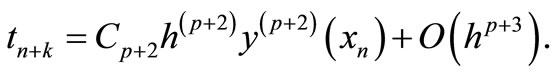 (15)
(15)
For our method,

Expanding in Taylor series gives

hence,


4. Zero Stability
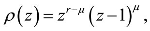
Definition 2. The block (2) is said to be zero stable, if the roots  of the first characteristic polynomial
  defined by
  satisfies
  have multiplicity not exceeding the order of the differential equation. Moreover as
 ,
,
 where
where  is the order of the differential equation, r is the order of the matrix
  and E (see [11] for details).
For our method

 ; hence our method is zero stable.
Region of Absolute Stability
Definition 3. The method (2) is said be absolutely stable if for a given value oh h, all the roots  of the characteristic polynomial
  satisfies
  where
where  and
and .
.
We adopted the boundary locus method for the region of absolute stability if the block method. Substituting the test equation  into the block formula gives


writing in trigonometric ratios gives
 (16)
(16)
where  Equation (16) is our characteristics polynomial (see [14] for details). Applying to our method

which gives the stability region to be [−14.35, 0] after evaluation  at interval of
  within [0, 180] The stability is shown in Figure 1.
5. Numerical Experiments
5.1. Test Problems
We test our scheme on second order initial value problems.
Problem 1: Consider the non linear initial value problem (I.V.P) which was solved by [11] using block method and [2] for step size  which is of order 8

Exact solution: 

Figure 1. Showing region of absolute stability of the block method.
We solved this problem using our method for stepsize h = 0.01. The result is shown in Table 1. Our method performed better than the methods compared with. This problem method was also solved [10] using block of lower order for h = 1/32. Though the details are not shown but our result performed better in term of accuracy.
Problem 2: Consider a linear second order initial value problem

Exact solution: .
.
This problem was also solved by [10]. The result in
Table 2 shows clearly that our method gives better approximation than the existing methods.
5.2. Numerical Results
The following notations are used in the table ESBK: Error in [11];
EAK: Error in [2];
EBK: Error in [10];
 .
.
6. Conclusion
We have proposed a non self starting continuous block method in this paper. It has been shown clearly that the non self starting method gives a better approximation than

Table 1. Showing results of problem 1.

Table 2. Showing results of problem 2.
the self starting method. The continuous parameter introduced in the block method allows evaluation at all points within the interval of integration; hence, it enables researchers to understand the behaviour of the system under investigation. We therefore recommend this new method when seeking for the solution of initial value problems.
NOTES