Unsteady Incompressible Flow of a Generalised Oldroyed-B Fluid between Two Infinite Parallel Plates ()
1. Introduction
The interest in studying problems involving non-Newtonian fluid flows has considerably grown for their wide range of applications. Visco-elastic fluids are described by various types of constitutive equations. Among them Oldroyed-B fluid model has some success in describing polymetric liquids. Recently, the fractional derivatives are found to be quite flexible in describing the behaviours of visco-elastic fluid and are studied by many mathematicians considering various motion of such fluids. In their studies, the constitutive equations for generalised non-Newtonian fluids are modified from the well known fluid models by replacing the time derivative of an integer order by the so-called Riemann-Liouville fractional calculus operators.
The practical applications of the fluid flow between two parallel plates are in the extraction and filtration of oils froms wells the drainage of water, irrigation, sanitary engineering, chemical engineering, food industry and also in the inter disciplinary fields such as biomedical engineering. Rajagopal and Gupta [1] studied a class of exact solutions to the equations of motion of a second grade fluid. Tan and Xu [2] investigated the impulsive motion of at plate in a general second grade fluid. KhanHayat and Agar [3] studied the exact solution for MHD flow of a generalized Oldroyed-B fluid with modified Darcy’s law. Tan and Masuoka [4] discussed Stokes first problem for a second grade fluid in a porous half-space with heated boundary. Qi and Xu [5] examined Stokes first problem for a viscoelastic uid with the generalized Oldroyd-B model. Fetecau, Khan, Fetecau and Qi [6] investigated exact solutions for the flow of a generalised Oldroyed-B fluid induced by a suddenly moved plate between two side walls perpendicular to the plate. Liu, Zheng, Zhang and Zong [7] discussed the oscillating flows and heat transfer of a generalised Oldroyed-B fluid in magnetic field.
The objective of this paper is to obtain exact solutions for a class of unsteady flows of a viscoelastic fluid involving the fractional derivative in time in the constitutive equation of Oldroyed-B fluid between two infinite parallel plates. The fractional calculus approach in the constitutive relationship model is introduced. In this case the governing equations of motion are of fractional order partial differential equations in place of second-order Navier-Stokes equations. By using the Laplace and the finite Fourier sine transformations, we obtain the exact solutions of the velocity fields of the fluid problems under consideration.
2. Mathematical Formulation
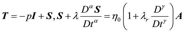
The constitutive equation of an incompressible and unsteady Oldroyed-B fluid can be written in the following form:
 (1)
(1)
where, T is the Cauchy stress tensor, p is the hydrostatic pressure, I is the identity tensor, S is the extra-stress tensor,  is the first Rivlin-Ericksen tensor, L is the velocity gradient,
  are material constants, known as the viscosity coefficient, the relaxation and retardation times respectively and α, γ are fractional parameters and
 (2)
(2)
 (3)
(3)
In the above relations V is the velocity vector,  is the gradient operator,
  and
and are Riemann-Liouville operators and defined by
 (4)
(4)
where, Γ(.) is the Gamma function.
Assuming the velocity field of the following form
 (5)
(5)
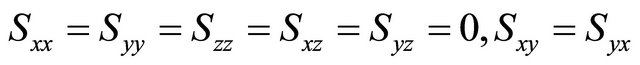
where u is the velocity component in the x-direction, i being the unit vector in the x-direction, xand y-axes are chosen along and perpendicular to the plates respectively. Substituting Equation (5) into Equation (1) and taking account of initial condition S(y, 0) = 0; y > 0, the fluid being at rest at t = 0,we get

 (6)
(6)
According to our problem,
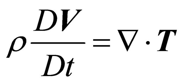
We consider a generalised Oldroyed-B fluid between two infinite parallel plates. Then in the absence of a pressure gradient in the x-direction, the equation of motion yields the following equation:
 (7)
(7)
where  is the density of the fluid and
  is the material derivative, T is the stress tensor, V denotes velocity vector.
The continuity equation is
 (8)
(8)
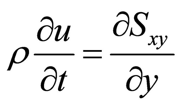
which is satisfied by the velocity vector, V = (u(y, t), 0, 0). Using the Equation (4) we get from Equation (6),
 (9)
(9)
Now eliminating  between Equations (6) and (9) we get the following governing equation of motion as
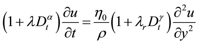 (10)
(10)
where,  is the kinematic viscosity.
Here we consider the unsteady incompressible viscoelastic flow of a generalised Oldroyed-B fluid between two infinite parallel plates. We consider the following two problems:
Problem 1: The flow between two parallel plates one of which is started moving suddenly and the other being at rest.
Problem 2: The flow between two parallel plates one of which is oscillating and the other being at rest.
Problem 1: The flow between two parallel plates one of which is started moving suddenly and the other being at rest.
For the present problem we take the velocity field of the form, V = u(y, t) i where, u is the velocity component in the x-cordinate direction, i is the unit vector in x- direction. x-and y-axes are chosen along and perpendicular to the plates respectively.
Let us consider the dimensionless variables:

where, “U” and “d” respectively denote the steady velocity of the moving plate and the distance between the plates.
Thus, the governing Equation (10) in nondimensional variables is given by:
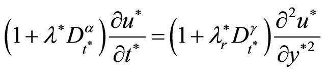
where, 
For simplicity, neglecting “*” mark, we get the governing equation in terms of nondimensional variables as follows:

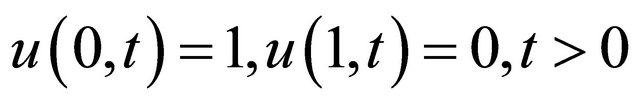
We suppose that an incompressible viscoelastic fluid is bounded by two infinite parallel plates, at a distance “d” apart. The x-axis is taken in the direction of the plates and y-axis is taken vertically upward. The plate at y = 0 is initially at rest and suddenly brought to the steady velocity “U” and then plate at y = d is always at rest.
Equation of motion of viscoelastic fluid is given by
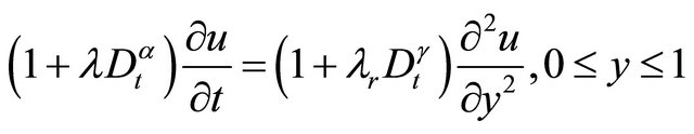 (11)
(11)
Initial conditions are given by

Boundary conditions in terms of non-dimensional variables can be written as

Now we introduce a transformation for variable u to v given by
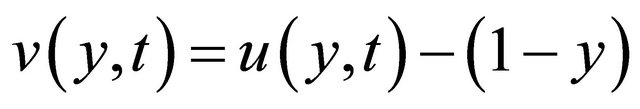 for t > 0 Then Equation (11) transform to
 (12)
(12)
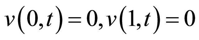
The initial condition is reduced to

and the boundary conditions are given by
Now multiplying both sides of Equation (12) by sin (nπy) and then integrating with respect to y from 0 to 1 and using boundary conditions we get,
 (13)
(13)
where,  is the finite Fourier sine transformation of
  and
and 
Taking Laplace transformation of both sides of Equation (13) and using  we get,
 (14)
(14)
where  is the Laplace transformation of
  with respect to t and p is the Laplace transform parameter.
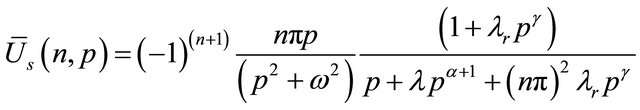
In order to avoid the lengthy procedure of residues and contour integrals, we rewrite Equation (14) into series form
 (15)
(15)
Now we have an important Laplace transformation of the nth order derivative of Mittage-Leffler function  given by
 (16)
(16)
where,  is the Mittag-Leffler function.

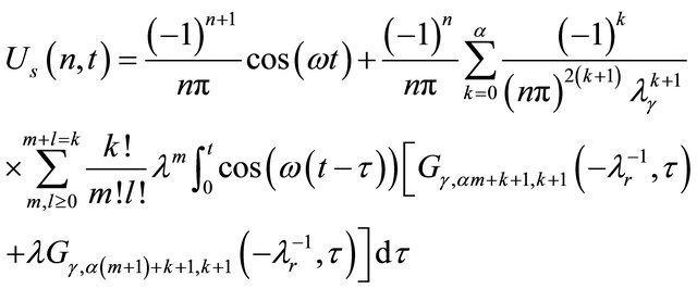
Taking discrete inverse Laplace transformation of Equation (15) we get
 (17)
(17)
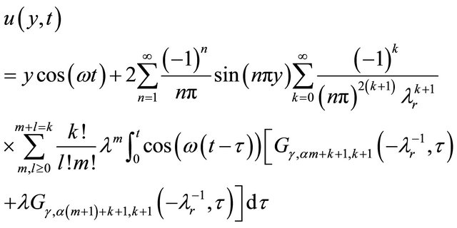
Taking discrete inverse finite Fourier sine transformation of the above equation we get,

Changing the variable  to
to  by the transformation
 , we get the expression for the velocity field as follows,
Problem 2: Flow between two infinite parallel plates in which upper plate oscillates and the lower plate being at rest.
Let us suppose that the distance between the two plates is “d”. The upper plate at y = d oscillates with dimensionless velocity  and the lower plate at y = 0 is at rest, where ω is the dimensionless frequency of the upper plate.
The governing equation is of the form given below
 (20)
(20)
where α, γ are the fractional parameters.
Initial condition is given by
Boundary conditions in term of dimensionless variables are given by

Now multiplying both sides of Equation (20) by sin(nπy) and then integrating with respect to y from 0 to 1 and using the boundary conditions we get,

where  is the finite Fourier sine transformation of u(y,t). Now taking the Laplace transformation of the above equation and using
  we get
where  is the Laplace transformation of
  and “p” is the Laplace transform parameter.
Now in order to avoid the lengthy procedure of residues and contour integrals, we rewrite the above equation into series form

Taking the discrete inverse Laplace transform of the above equation we obtain,
 (22)
(22)
where  is the Generalised function and
  is the Pochhammer polynomial.
Now taking discrete inverse finite Fourier Sine transformation we get from Equation (22) the velocity field as
 (23)
(23)
3. Limiting Cases
Case 1: If ,
,  , then the equation of motion and the boundary conditions are:
 (24)
(24)
with boundary conditions: u(0, t) = 1, u(1, t) = 0, for t > 0 for the Problem 1 and u(0, t) = 0, u(1, t) = cos(ωt) for t > 0 for the Problem 2.
The Equation (24) represents the governing equation for a classical Newtonian fluid.
Case 2: If γ ≠ 0,  , the solutions for a generalised Maxwell fluid is recovered from the solutions given by the Equations (18) and (23).
Case 3: If α ≠ 0, λ→0, then the equation the equation of motion is
 (25)
(25)
with boundary conditions: u(0, t) = 1, u(1, t) = 0, t > 0 for the Problem 1 and u(0, t) = 0, u(1, t) = cos(ωt), t > 0 for the Problem 2 Equation (25) represents the governing equation for a Generalised Second Grade fluid.
Case 4: If ,
,  , the solutions for an ordinary Oldroyed-B fluid is recovered from the solutions given by the Equations (18) and (23).
4. Conclusions and Numerical Results
In this paper we have presented some unsteady incompressible flow of a generalized Oldroyed-B fluid between two infinite parallel plates in two different problems. Exact analytical solutions are obtained for the velocity fields by means of Laplace and finite Fourier sine transformations in series form in terms of Mittag-Leffler function  and generalised function,
 . In the constitutive model, the time derivative of integer order is replaced by Riemann-Liouville operator given by Equation (4). The four limiting cases of the general solutions have been discussed in the paper. The diagrams have been drawn against t for different values of the fractional parameters α and γ. The influence of the fractional parameters upon the velocity field has been discussed graphically.
1) Problem 1 In Figure 1 the velocity is depicted against the distance from the lower plate. The fluid velocity increases in the region between the widths y = 0.0 and 0.8 with the increase in time. The velocity curves are smooth in character. The velocity profile has some deviation from parabolic pattern depending on the time t. In Figure 1

Figure 1. The velocity is depicted against the distance from the lower plate. λr = 3, λ = 5, α = 0.2, γ = 0.8.

Figure 2. The velocity is depicted against time with different values of fractional parameter γ. y = 0.1, λr = 3, λ = 5, α = 0.2.
we have a point of local minimum value in the velocity curve of t = 2, because the velocity gradient at that point(near the midway of the two parallel plates) is zero.
In Figure 2 we can see the dependency of the velocity profile on the fractional parameter γ. As the value of the parameter γ increases, the fluid velocity decreases with time near the lower plate and as the time progresses the fluid flow increases with the increase of value of γ near the lower plate. In Figure 3 the velocity field has been depicted against time with different values of fractional parameter α. The Figure shows the dependency of the velocity field on the fractional parameter α. The flow velocity increases with the increasing values of the frac-

Figure 3. The velocity is depicted against time with different values of fractional parameter α. y = 0.1, λr = 3, λ = 5, γ = 0.8.
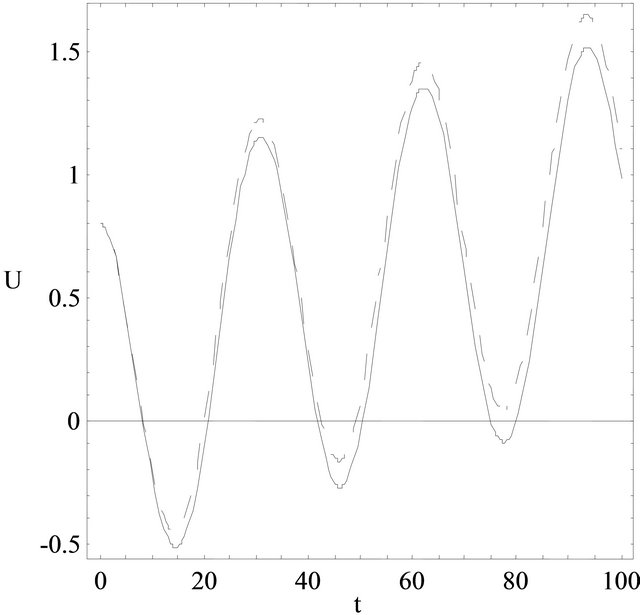
Figure 4. The velocity is depicted against time near the upper plate with different values of fractional parameter, α. ω = 0.2, λr = 5, λ = 3, γ = 0.8, y = 0.9. : α = 0. 2; _____: α = 0.4.
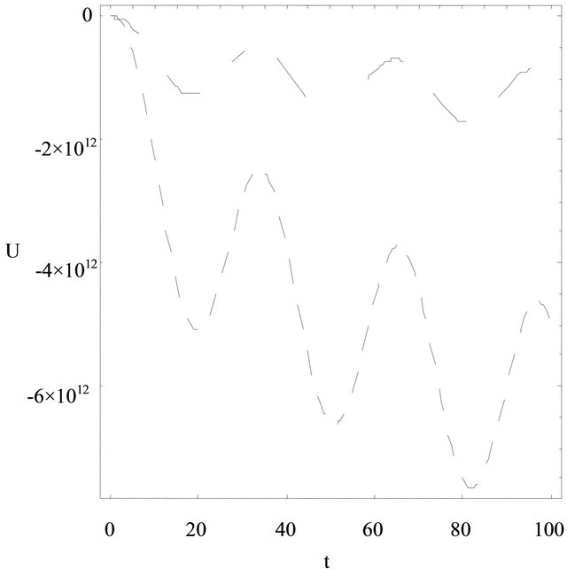
Figure 5. The velocity is depicted against time for two cases. 1) Classical newtonian fluid; 2) Generalised Maxwell fluid. 1) ω = 0.2, λr = 0.0001, λ = 3, α = 0.0, γ = 0.8, y = 0.8. Classical newtonian fluid _ _ _ _ _; 2) ω = 0.2, λr = 0.0001, λ = 3, α = 0.2, γ = 0.8, y = 0.8, generalised maxwell fluid ___ ____.
tional parameter α. In all the cases, the velocity increases with the increase in time.
2) Problem 2 In Figure 4 the velocity is plotted against time, t for different values of fractional parameter, α. The fluid velocity decreases with the increasing values of parameter α. For different values of α, the central line of the oscillation is deviating from the horizontal line with respect to time in Figure 4. This effect is seen after lapse of long time. In Figure 5, the velocity is depicted against time for two cases: Case 1, classical Newtonian fluid; and Case 2, generalised Maxwell fluid for the Problem 2. In Case 1,  and in Case 2
 ,
, ≠ 0. From Figure 5, it can be concluded that the velocity curves in both the cases are oscillatery in nature and the fluid velocity for Classical Newtonian fluid decreases negatively with oscillation compare to the flow for Generalised Maxwell fluid near the upper plate. The central lines of oscillation for both the cases shift downwards the time axis.
NOTES