Numerical Solution of Troesch’s Problem by Sinc-Collocation Method ()
1. Introduction
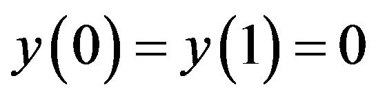
In this paper, we consider a two-point boundary value problem, Troesch’s problem [1-3], defined by
 (1)
(1)
 (2)
(2)
where  is a positive constant. This problem arises in an investigation of the confinement of a plasma column by radiation pressure [4] and also in the theory of gas porous electrodes [5,6]. This problem has been studied extensively. Troesch found its numerical solution in [7] using the shooting method, in [8] using the decomposition technique, in [9-11] using the variational iteration method, in [12] using a combination of the multipoint shooting method with the continuation and perturbation technique, in [13] using the quasilinearization method, in [14] using the method of transformation groups, in [15] the invariant imbedding method, in [16] using the inverse shooting method, in [17] using the modified homotopy perturbation method, in [18] using sinc-Galerkin method, in [19] using B-spline method, in [20] using the differential transform method and in [21] using chebychev collocation method.
The purpose of this paper is to introduce a novel approach based on sinc function for the numerical solution of the class of nonlinear boundary value problems given in (1)-(2). Sinc approximation have become increasingly important in numerical analysis. Most commonly used techniques with sinc-collocation have been examined in [22-24] and references therein. The error of the method converges to zero like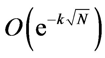 , as
, as , where N is the numerical of collocation points used, and where k is a positive constant independent of N.
The aim of this work is two folds. First we aim to investigate the ODEs of a variety of distinct orders, linear or nonlinear, to show that sinc-collocation method can work as a unified method. Second we aim to confirm the power of the sinc-collocation method in handling scientific and engineering problems.
The remaining structure of this article is organized as follows: a brief introduction to the sinc function is presented in Section 2. In Section 3, the sinc-collocation approach for the solution of Troesch’s problem is described. The results are compared with the exact solutions and some existing numerical solutions in Section 4. Finally, in Section 5, a conclusion is given that briefly summarizes the results.
2. Sinc Function
A general review of sinc function approximation is given in [25,26] and the recent papers [27-29]. Hence, only properties important to the present goals are outlined in this section.
If  is defined on the real line, then for
  the Whittaker cardinal expansion of f
where , and the mesh size is given by
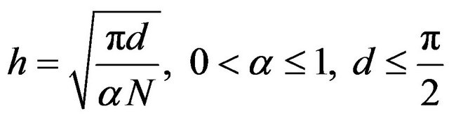 (3)
(3)
where N is suitably chosen and  depends on the asymptotic behavior of
 . The basis functions on
  are then given by
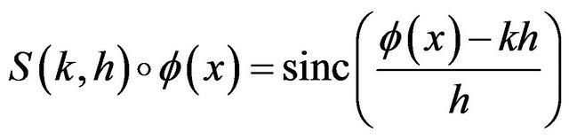
and
 (4)
(4)
The interpolation formula for  over
over  takes the form
 (5)
(5)
The n-th derivative of the function  at points
 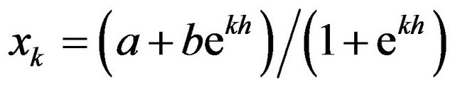 can be approximated using a finite number of terms as
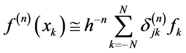 (6)
(6)
where

The quadrature formula of  is given by
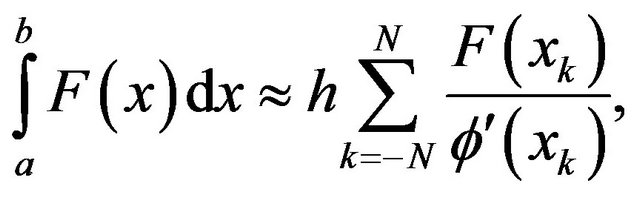 (7)
(7)
We consider the following definitions and theorems in [26].
Definition 1.
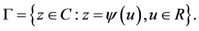
Let  be a simply-connected domain in the complex
  plane having boundary
 . Let
. Let  and
and  denote two distinct points of
  and
and  denote a conformal map of
  onto
onto , where
  denote the region
such that  and
and . Let
. Let  denote the inverse map, and let
  be defined by
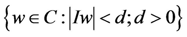
Given  and a positive number
  let us set
 , let us also
  by
by .
.
Definition 2.
Let  be the set of all analytic functions, for which there exists a constant,
  such that

Theorem 1.
Let , let
, let  be a positive integer, and
  be selected by the Formula (3) then there exist positive constant
 , independent of
 , such that
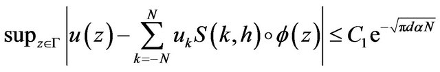 .
.
3. The Description of Sinc-Collocation Scheme
First, the sinc function composed with various conformal mappings,  , are zero at the endpoints of the interval. Since the boundary conditions are nonhomogeneous, then these conditions need be converted to homogeneous ones via an interpolation by a known function. The nonhomogeneous boundary conditions in (2) can be transformed to homogeneous boundary conditions by the change of dependent variable
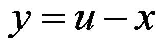 . The new problem with homogeneous boundary conditions is then
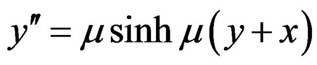 (8)
(8)
subject to the boundary conditions
 (9)
(9)
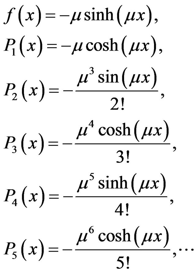
To obtain its approximate solution of Equations (8) and (9), we expand  around

Particularly, if , then

and
The Equation (8) becomes
 (10)
(10)
where
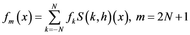
The approximate solution for  is represented by the formula
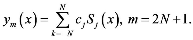 (11)
(11)
We need the following lemma.
Lemma.
The following relation holds
 (12)
(12)
where N and  are now dependent on both
  and
and .
.
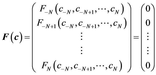
Replacing the terms of (10) with the appropriate representation defined in (5), (6), and (12) and applying the collocation to it, we eventually obtain the following theorem.
Theorem 2.
If the assumed approximate solution of problem (10) and (9) is (11), then the discrete sinc-collocation system for the determination of the unknown coefficients is given by
 (13)
(13)
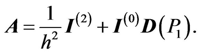
The following notation will be necessary for writing down the system. Let  be the
  diagonal matrix
 (14)
(14)
and define the  matrices
  (see [30]) for
  by
by
 (15)
(15)
whose kj-th entry is given by

Let c be the m-vector with j-th component given by , let
, let  be the m-vector with j-th component given by
 , and 1 is an m-vector each of whose components is 1. In this notation the system in (13) takes the matrix form
 (16)
(16)
where
and
Now we have a nonlinear system of  equation of the m unknown coefficients, namely,
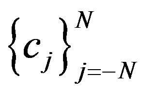 .
.
We can obtain the coefficient of the approximate solution by solving this nonlinear system by Newton’s method. The solution 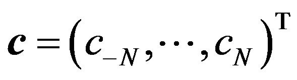 gives the coefficients in the approximate sinc-collocation solution
  of
of . Then, the approximate solution of (1) is

Newton’s Method.
To solve the system of Equation (16), we express these equations as the simultaneous zeroing of a set of functions, where the number of functions to be zeroed is equal to the number of independent variables.
 (17)
(17)
A very important method for the solution of Equation (17) is Newton’s method:
Let  be the guess at the solution for iteration i. Assuming the
  is not small enough, we seek an update vectors
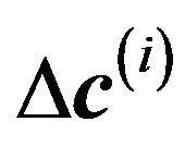
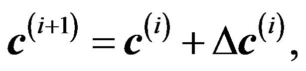
i.e.
 (18)
(18)
such that . Using the multidimensional extension of Taylor’s theorem to approximate the variation of
 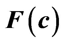 in the neighborhood of
  gives
gives
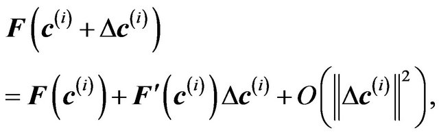 (19)
(19)
where  is the Jacobian of the system of equations:
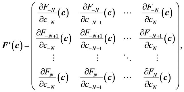 (20)
(20)
Neglecting higher order terms and designating  as the Jacobian evaluated at
 . We can rearrange Equation (19)
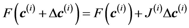 (21)
(21)
The goal of Newton iterations is to make  , so setting that term to zero in the preceding equation gives
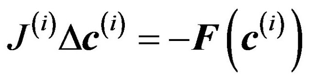 (22)
(22)
Equation (22) is a system of m linear equations in the m unknown . Each Newton iteration step involves evaluation of the vector
 , the matrix
  and the solution to Equation (22). A common numerical practice is to stop the Newton iteration whenever the distance between two iterates is less than a given tolerance, i.e. when

• Algorithm.
• Initialize: 
• For 
• 
• If  is small enough, stop
• Compute 
• Solve 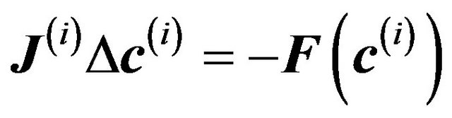
• 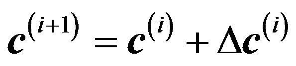
• End.
4. Numerical Examples
The closed form solution to this problem in terms of the Jacobian elliptic function has been given [3] as
 (23)
(23)
where , the derivative of
  at 0, is given by the expression
 , with
  being the solution of the transcendental equation
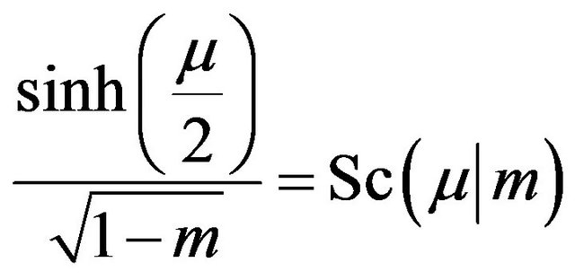
where the Jacobian elliptic function  [2,31] is defined by
  where
where  and
and  are related by the integral

In Tables 1 and 2 the numerical solution obtained by sinc-collocation method is compared with the exact solution derived from Equation (23) and with the numerical solution obtained by the modified homotopy perturbation technique (MHP) [17], variation method [9] and decomposition method [8] for the case  and
and  respectively .
In Table 3, the numerical solution obtained by the sinc-collocation method for  is compared with the numerical approximation of the exact solutions given by a Fortran code called TWPBVP and the numerical solution obtained by B-spline collocation method [19].
5. Discussions
There are two main goals that we aimed for this work. The first is to employ the powerful sinc-collocation method to investigate nonlinear ordinary differential equations. The second is to show the power of this method and its significant features. The two goals are achieved.
In [27], we compared the performance of the collocation and Galerkin methods using sinc bases for solving linear and nonlinear second order two-point boundary value problems and shown that the most significant virtue
Table 1. Numerical solutions of Troesch’s problem for the case μ = 0.5.

Table 2. Numerical solutions of Troesch’s problem for the case μ = 1.
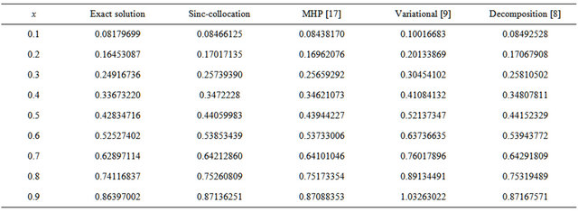
Table 3. Numerical solutions of Troesch’s problem for the case μ = 5.

of the collocation procedure is its ease in application. The collocation method easily generalizes to problems having general boundary conditions.