The Statistical Analysis of Interval-Censored Failure Time Data with Applications ()
1. Introduction
A great many studies in statistics deal with deaths or failures of components: they involve the numbers of deaths, the timing of death, or the risks of death to which different classes of individuals are exposed. The analysis of survival data is a major focus of statistics.
In standard time-to-event analysis, the time to a particular event of interest is observed exactly or right-censored. Numerous methods are available for estimating the survival curve and also for estimation of the effects of covariates for these cases. In certain situations, the times of the event of interest may not be exactly known. This means that it may have occurred within particular time duration. In clinical trials, patients are often seen at pre-scheduled visits but the event of interest may have occurred in between visits. These types of data are known as interval-censored data.
Right-censored data can be considered as a special case of interval-censored data. Some of the inference approaches for right-censored data can be directly, or with minor modifications, used to analyze interval-censored data. However, most of the inference approaches for right-censored data are not appropriate for interval-censored data due to fundamental differences between these two types of censoring. The censoring approach behind interval censoring is more complicated than that of right censoring. For right-censored failure time data, substantial advances in the theory and development of modern statistical methods are based on the counting processes theory, which is not applicable to interval-censored data. Due to the complexity and special structure of interval censoring, the same theory is not applicable to interval-censored data.
Interval censoring has become increasingly common in the areas that produce failure time data. Over the past two decades, a lot of literature on the statistical analysis of interval-censored failure time data has appeared.
Lindsay and Ryan [1] provided a tutorial on Biostatistical methods for interval-censored data. This paper illustrated and compared available methods which correctly treated the data as being interval-censored. This paper did not provide a full review of all existing methods. However, all approaches were illustrated on two data sets and compared with methods which ignore the interval-censored nature of the data. In this paper, we have used some of the methodologies, notations and equations used by Lindsay and Ryan [1].
Lindsay [2] showed that parametric models for interval censored data can now easily be fitted with minimal programming in certain standard statistical software packages. Regression equations were introduced and finite mixture models were also fitted. Models based on nine different distributions were compared for three examples of heavily censored data as well as a set of simulated data. It has been found that interval censoring can be ignored for parametric models. Parametric models are remarkably robust with changing distributional assumptions and more informative than the corresponding non-parametric models for heavily interval censored data.
Finkelstein and Wolfe [3] provided a method for regression analysis to accommodate interval-censored data. Finkelstein [4] develops a method for fitting proportional hazards regression model when the data contain intervalcensored observations. The method described in this paper is used to analyze data from an animal study and also a clinical trial.
Peto [5] provided a method of calculating an estimate of the cumulative distribution function from intervalcensored data, which was similar to the life-table technique.
Rosenberg [6] presented a flexible parametric procedure to model the hazard function as a linear combination of cubic B-Splines and derived maximum likelihood estimates from censored survival data. This provided smooth estimates of the hazard and survivorship functions that are intermediate between parametric and non-parametric models. HIV infections data that were intervalcensored were used to illustrate the methods.
Odell et al. [7] studied the use of a Weibull-based accelerated failure time regression model when intervalcensored data were observed. They have used two alternative methods to analyze the data. Turnbull [8] has used non-parametric estimation of a distribution function for censored data. A simple algorithm using self-consistency as a basis was used to get maximum likelihood estimates.
Farrington [9] provided a method for weak parametric modeling of interval-censored data using generalized linear models. Three types of models, namely, additive, multiplicative and proportional hazard model with discrete baseline survival function were considered. Goetghebeur and Ryan [10] introduced semi-parametric regression analysis of interval censored data. A semi-parametric approach to the proportional hazards regression analysis of interval-censored data was proposed in this paper. The method was illustrated on data from the breast cancer cosmetics trial, previously analyzed by Finkelstein [4].
Lawless [11] provides a unified treatment of models and statistical methods used in the analysis of lifetime or response time data (Chapter 3, Section 3.5.3, p. 124). Numerical illustrations and examples involving real data demonstrate the application of each method to problems in areas such as reliability, product performance evaluation, clinical trials, and experimentation in the biomedical sciences. Collet [12] describes and illustrates the modeling approach to the analysis of survival data. Some methods for analyzing interval-censored data are described and illustrated. This begins with an introduction to survival analysis and a description of four studies in which survival data was obtained. These and other data sets then illustrate the techniques presented, including the Cox and Weibull proportional hazards models, accelerated failure time models, models with time-dependent variables, interval-censored survival data and model checking.
Sun [13] has recently presented statistical models and methods specifically developed for the analysis of interval-censored failure time data. This book collects and unifies statistical models and methods that have been proposed for analyzing interval-censored failure time data. It provides the first comprehensive coverage of the topic of interval-censored data. This focuses on non-parametric and semi-parametric inferences, but it also describes parametric and imputation approaches. This paper reviews the substantial body of recent work in this field and also provides some applications.
2. Statistical Methodology
2.1. Parametric Methods
The straightforward procedure to analyze censored data is to assume a parametric model for the failure times. It is possible to fit Accelerated failure time (AFT) models for a variety of distributions to interval censored data. In the statistical area of survival analysis, an accelerated failure time model is a parametric model that provides an alternative to the commonly-used proportional hazards models. A proportional hazards model assumes that the effect of a covariate is to multiply the hazard by some constant; an AFT model assumes that the effect of a covariate is to multiply the predicted event time by some constant. AFT models can therefore be framed as linear models for the logarithm of the survival time.
The results of AFT models are easily interpreted. For example, the results of a clinical trial with mortality as the endpoint could be interpreted as a certain percentage increase in future life expectancy on the new treatment compared to the control. So a patient could be informed that he would be expected to live (say) 15% longer if he took the new treatment. Hazard ratios are harder to explain in layman’s terms. More probability distributions can be used in AFT models than parametric proportional hazards models. A distribution must have a parameterization that includes a scale parameter to be used in an AFT model. The logarithm of the scale parameter is then modeled as a linear function of the covariates.
The Weibull distribution (including the exponential distribution as a special case) can be parameterized as either a proportional hazards model or an AFT model, and is the only family of distributions to have this property. The results of fitting a Weibull model can therefore be interpreted in either framework. Unlike the Weibull distribution, log-logistic distribution can exhibit a non-monotonic hazard function which increases at early times and will decrease at later times.
Other distributions suitable for AFT models include the log-normal and log-gamma distributions, although they are less popular than the log-logistic, partly as their cumulative distribution functions do not have a closed form.
The SAS procedure LIFEREG provides a way of fitting accelerated failure time models for a variety of distributions to interval censored data. The AFT model is defined by the transformation
 , (2.1)
where  is the failure time random variable for an individual with covariate z and
  is the failure time that the individual would have if they had covariate value 0. The effect of changing covariates is to shrink or stretch the time to event. If
  is negative, then the covariate has the effect of “speeding up time” so that individuals with larger values of z have higher failure rates and hence shorter survival times. The survival function can be written as
 , (2.2)
where  is the survival function for an individual with covariate value 0. Taking natural logarithm, the AFT model can be expressed as
 . (2.3)
If we assume that  can be expressed as
 , where W is a random variable, then the model can be written in a linear model-like form:
 . (2.4)
The PROC LIFEREG module of SAS fits this model, except that the sign is changed on the regression coefficients. That is, SAS fits
 . (2.5)
It is possible to include a variety of distributions to be placed on the error term W with SAS, including the log of the exponential, log-normal and log-gamma distributions. The intercept parameter  and the scale parameter
  are usually not of direct interest, although for some distributions, there is a relationship between the AFT model and a proportional hazards model through the scale parameter. For example, if W is an extreme value distribution (log of a unit exponential), then T has a Weibull distribution. Note that because of the change in sign implicit in the AFT formulation, the direction of covariate effects will be opposite to those fit with a Cox proportional hazards model.
2.2. Non-Parametric Estimation of Survival Curve
2.2.1. Kaplan-Meier Estimator
The Kaplan-Meier estimator estimates the survival function for life-time data. In medical research, it might be used to measure the fraction of patients living for a certain amount of time after treatment. An economist might measure the length of time people remain unemployed after a job loss. An engineer might measure the time until failure of machine parts.
A plot of the Kaplan-Meier estimate of the survival function is a series of horizontal steps of declining magnitude which, when a large enough sample is taken, approaches the true survival function for that population. The value of the survival function between successive distinct sampled observations is assumed to be constant.
An important advantage of the Kaplan-Meier curve is that the method can take censored data into account, for instance, if a patient withdraws from a study. When no truncation or censoring occurs, the Kaplan-Meier curve is equivalent to the empirical distribution.
Let  be the probability that an item from a given population will have a lifetime exceeding t. For a sample from this population of size N let the observed times until death of N sample members be
 . (2.6)
Corresponding to each  is
is , the number “at risk” just prior to time
 , and
, and , the number of deaths at time
 .
.
Note that the intervals between each time typically will not be uniform. For example, a small data set might begin with 10 cases, have a death at Day 3, a loss (censored case) at Day 9, and another death at Day 11. Then we have ,
,  , and
, and .
.
The Kaplan-Meier estimator is the nonparametric maximum likelihood estimate of . It is a product of the form
 . (2.7)
When there is no censoring,  is just the number of survivors just prior to time
 . With censoring,
  is the number of survivors less the number of losses (censored cases). It is only those surviving cases that are still being observed (have not yet been censored) that are “at risk” of an (observed) death.
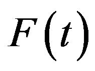
Let T be the random variable that measures the time of failure and let  be its cumulative distribution function. Note that
 (2.8)
(2.8)
Consequently, the right-continuous definition of  may be preferred in order to make the estimate compatible with a right-continuous estimate of
 .
.
With right-censored data, Kaplan and Meier [14] showed that the closed form product limit estimator is the generalized maximum likelihood estimate. This curve jumps at each observed event time.
2.2.2. Turnbull Estimator
In most applications, the data may be interval-censored. By interval-censored data, a random variable of interest is known only to lie in an interval, instead of being observed exactly. In such cases, the only information available for each individual is that their event time falls in an interval, but the exact time is unknown. A nonparametric estimate of the survival function can also be found in such interval censored situations. The survival function is perhaps the most important function in medical and health studies. In this section, the iterative procedure proposed by Turnbull [8] to estimate such function is described and illustrated.
Situations where the observed response for each individual under study is either an exact survival time or a censoring time are common in practice. Other situations, however, can occur, and amongst them we find the longitudinal studies, where the individuals are followed for a pre-fixed time period or visited periodically for a fixed number of times. In this context, the time  until the occurrence of the event of interest for each individual is only known (whenever it occurs) to be within the interval between visits, i.e., between the visit in time
  and the visit in time
 . Note that in such studies, the survival times
  are no longer known exactly. It is only known that the event of interest has occurred within the interval
 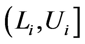 with
with . Furthermore, note that if the event occurs exactly at the moment of a visit, which is very improbable but can happen, then we have an exact survival time. In this case it is assumed that
 .
.
On the other hand, it is known for the individuals with right censoring that the event of interest did not occur until the last visit but it can happen at any time from that moment on. We therefore assumed in this case that  can occur within the interval
  with
with  being equal to the period of time from the beginning of the study until the last visit and
 .
.
Similarly, it is known for the individuals that are left censored, that the event of interest has occurred before the first visit and, hence, we assume that  falls in the interval
  with
with  representing the beginning of the study and
 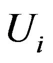 is the period of time from the beginning of the study until the first visit.
Note from what we have presented so far that exact survival times as well as right and left censored data, are all special cases of interval survival data with  for exact times,
 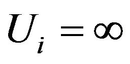 for right censoring and
  for left censoring. We can therefore state that interval survival data generalize any situation with combinations of survival times (exact or interval) and right and left censoring that can occur in survival studies.
As usual in the analysis of non-interval survival data, it is also of interest to estimate the survival function  and to assess the importance of potential prognostic factors. Few statistical software allow for such data, and for this reason a common practice amongst data analysts is to assume that the event occurring within the interval
  has occurred either at the upper/lower limit of the interval or, at the middle point of each interval. Rucker and Messerer [15], Odell et al. [7] and Dorey et al. [16] stated that assuming interval survival times as exact times can lead to biased estimates as well as results and conclusions that were not fully reliable. In this work we describe a nonparametric procedure for estimation of the survival function for interval survival data.
Peto [5] was the first to propose a non-parametric method for estimating the survival distribution based on interval-censored data. Turnbull [8] derived the same estimator, but used a different approach in estimation. Suppose , the survival times for n patients, are independent random variables with right continuous survival function
 . If
. If  are not observed directly, but instead are known to lie in the interval
 , then the likelihood for the n observations is,
 . (2.9)
By , we mean
 (2.10)
which may be different from , since
  is left continuous. It is important to note that different authors vary in their conventions regarding definition of the censoring interval. The Convention of Peto [5] and Turnbull [8] who assumed a closed interval,
  , was followed. This definition facilitates the accommodation of observations that are known exactly, that is,
  , but necessitates the use of the
  notation in above Equation (2.9) to allow a non-zero contribution to the likelihood for these observations. Finkelstein [4] assumed semiclosed censoring intervals, which need to add the convention that the likelihood contribution for any observation with an exact failure time,
  , is
, is . Good arguments against almost any convention can be made for defining the censoring intervals. In practice, the choice will have little impact and all reasonable conventions can be adopted.
Turnbull [8] derived the same estimator using an iterative self-consistency algorithm, described below. Gentleman and Geyer [17] showed that this self-consistent estimator is not always the maximum likelihood estimator (MLE), and that the MLE is not necessarily unique and discuss conditions under which this can be determined.
Since the observed event times are known to occur only within potentially overlapping intervals, the survival curve can only jump within so-called equivalence sets ,
,  , where
 . The curve between
  and
and  is flat. The estimate of
 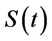 is unique only up to these equivalence classes; any function that jumps the appropriate amount within the equivalence class will yield the same likelihood.
An analog of the Product-Limit estimator of the survival function for interval-censored data is presented in this section. This estimator, which has no closed form, is based on an iterative procedure and has been suggested by Turnbull [8].
To construct the estimator, let  be a grid of time which includes all the points
  and
and  for
for . For the
  observation, define a weight
  to be 1 if the interval
  is contained in the interval
  and 0, otherwise. The weight
 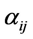 indicates whether the event which occurs in the interval
  could have occurred at
 . An initial guess at
  is made and Turnbull’s algorithm is as follows:
Step 1: Compute the probability of an event occurring at time  by
by
 (2.11)
Step 2: Estimate the number of events which occurred at  by
by
 (2.12)
Step 3: Compute the estimated number at risk at time
 by
by 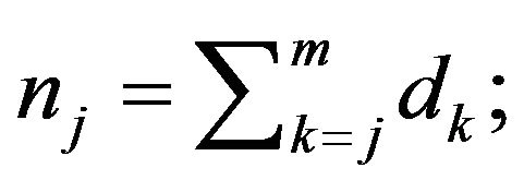
Step 4: Compute the updated Product-Limit estimator using the pseudo data found in Steps 2 and 3. If the updated estimate of S is close to the old version of S for all ’s, stop the iterative process, otherwise repeat Steps 1- 3, using the updated estimate of S.
2.2.3. Logspline Estimation of the Survival Curve
Kooperberg and Stone [18] have introduced the Logspline density estimation. They have developed a system for data that may be right censored, left censored, or interval censored. A fully automatic method was used to determine the estimate, which involved the maximum likelihood method and may involve stepwise knot deletion and either the Akaike information criterion (AIC) or Bayesian information criterion (BIC), was used to determine the estimate.
Kooperberg and Stone [18] provided software (logspline. fit, available through Statlib for S-plus2) which can be used to obtain smoothed estimates of the survival function based on interval censored data using splines. Smooth functions were fitted to the log-density function of the failure times within subsets of the time axis defined by the “knots”, and constrained to be continuous at those points. This provides a loosely parametric framework for finding estimates of the survival and hazard functions which can be useful for exploratory data analysis. Their approach is related to that of Rosenberg [6] who uses splines to model the hazard function.
3. Applications
There are essentially three approaches to fit survival models. The first straightforward method is the parametric approach, where a specific functional form for the baseline hazard 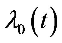 is assumed. Examples are: models based on the exponential, Weibull, gamma and generalized F distributions. A second approach might be called a flexible or semi-parametric strategy, where mild assumptions are made about the baseline hazard
 . Specifically, time is subdivided into reasonably small intervals and it is assumed that the baseline hazard is constant in each interval leading to a piecewise exponential model. The third approach is a non-parametric strategy that focuses on estimation of the parameters leaving the baseline hazard
  completely unspecified. This approach relies on a partial likelihood function proposed by Cox [19].
Five ways of estimating the time to event ignoring the effects of covariates are considered initially. Standard Kaplan-Meier estimator is used first. It is assumed that exact times of event are known and this is done either by assuming the event occurred at the left interval, or at the right interval. These two extreme cases should roughly bracket the estimates derived using the interval-censoring methods. A second approach is using a Weibull model, where the survivals function is modeled using the estimates from the SAS Proc LIFEREG. A Third procedure is to model the interval-censored nature of the data using the techniques proposed by Turnbull. The fourth is to use splines models proposed by Kooperberg and Stone [18]. Finally, the survival function is estimated using the piecewise exponential model.
3.1. Breast Cancer Data
This data set is from a retrospective study of patients with breast cancer designed to compare radiation therapy alone versus in combination with chemotherapy with respect to the time to cosmetic deterioration. This data set has been analyzed by several authors to illustrate various methods for interval censored data. Patients were seen initially every 4 to 6 months, with decreasing frequency over time. If deterioration was seen, it was known only to have occurred between two visits. Deterioration was not observed in all patients during the course of the trial, so some data were right-censored.
The breast cancer data set is described in detail in Finkelstein and Wolfe [3] and it consists of a total of 94 observations from a retrospective study looking at the time to cosmetic deterioration. Information is available on one covariate, type of therapy, either radiation alone (coded 0), or in combination with chemotherapy (coded 1). Of the 94 observations, 56 are interval-censored and 38 are right-censored. All estimated curves for the Breast Cancer data are presented in Figure 1. KM for R and KM for L represent Kaplan Meier estimates for right censored and left censored data respectively in Figures 1-3.
3.2. AIDS Data
This data set focused on the development of drug resistance (measured using a plaque reduction assay) to zidovudine in patients enrolled in four clinical trials for the treatment of AIDS. Samples were collected on the patients at a subset of the scheduled visit times dictated by the four protocols. Since the resistance assays were very expensive, there were few assessments on each patient, resulting in very wide intervals, 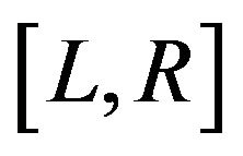 , if resistance was seen to have occurred, and a high proportion of right-censored observations. Because of the sparseness of these data, this is a challenging data set to analyze. The variables of interest were the effects of stage of disease,

Figure 1. All estimated curves for the breast cancer data.
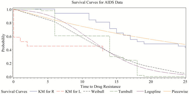
Figure 2. All estimated curves for AIDS data.

Figure 3. All estimated curves for hemophilia data.
dose of zidovudine and CD4 lymphocyte counts at time of randomization on the time to development of resistance. All estimated curves for the AIDS data are presented in Figure 2.
Lindsay and Ryan [1] have presented both Breast Cancer and AIDS data sets. More information about these two data sets could be found there. Some of the analyticcal methods, notations and results presented in this paper are similar to their paper.
3.3. Hemophilia Data
In 1978, 262 persons with Type A or B hemophilia have been treated at Hospital Kremlin Bicetre and Hospital Coeur des Yvelines in France. Twenty-five of the hemophiliacs were found to be infected with HIV on their first test for infection. By August 1988, 197 had become infected and 43 of these had developed clinical symptoms (AIDS, lymphadenopathy, or leukopenia) relating to their HIV infection. All of the infected persons were believed to have become infected by contaminated blood factor received for their hemophilia. The observations for the 262 patients were based on a discretization of the time axis into 6-month intervals. Here time is measured in 6-month intervals, with L = 1 denoting July 1, 1978, and Z denoting chronologic time of first clinical symptom. The 25 hemophiliacs infected at entry are assigned L = 1. Victor and Stephen [20] have presented this data in their paper and more information could be found there. They have initially analyzed Hemophilia data considering this as a Doubly-Censored Survival Data. However, we have analyzed this data set taking left censoring, right censoring and interval censoring into consideration. All estimated curves for the Hemophilia data are presented in Figure 3.
For the breast cancer example, the Kaplan-Meier estimates, bracket the Turnbull estimate. The Turnbull curve lies very close to both Weibull and logspline curves. At the same time, estimates from the Weibull, and logspline estimates are quite close to each other. The piecewise curve does not properly fall within the Kaplan-Meier estimates.
The estimated survival curve for the AIDS data took very few steps in the non-parametric models, which reflected the high degree of censoring in this small data set. The Kaplan-Meier estimates no longer bracketed the Turnbull estimate, mainly because the Turnbull estimate had very few jumps due to the particular configuration of this data set. The logspline estimate also tracked the parametric models closely. The non-parametric methods were not very helpful in understanding the AIDS data.
For the Hemophilia data, the results were quite similar to breast cancer data except the logspline model. Results derived for the piecewise exponential are not accurate for all three data sets.
3.4. Covariate Effects on Time to Event
To compare the two treatments, for Breast cancer data a retrospective study of 46 radiation only and 48 radiation plus chemotherapy patients was conducted. Using Turnbull’s algorithm the estimated survival functions were obtained for radiotherapy only and radiation plus chemotherapy groups respectively, which are shown in Figure 4. Note that the estimated survival curves did not show striking differences from 0 to 18 months. From 18 onwards, however, a fast decay of the curve is seen for patients given radiotherapy plus chemotherapy. Note, for instance, that only 11.06% of the patients in the radiotherapy plus chemotherapy group were estimated to be free of any evidence of breast retraction at time t = 40 months against 47.37% in the radiotherapy group.
Using the midpoint of each interval, is a common practice among analysts due to the lack of well-known statistical methodology and available software. Then applying the Kaplan-Meier method, we obtained the estimated survival curves presented in Figure 5. The curves estimated previously are also shown in the graph. Comparing the curves we can see that the estimates obtained using both, the midpoints and the intervals, are very similar to each other at several times but they tend to be under or over estimated at others. Although not shown here, under or over estimation became more evident if it is assumed that the event occurred to the end or at the beginning of each interval instead of at the midpoint. The range of each interval also contributes for the magnitude of these differences. They are more accentuated as the range of each interval increases.
Positive parameter estimates in Cox regression indicate higher failure rates for individuals with larger values of the covariate. The exponential model parameter should be of comparable magnitude to the Cox model, but with the sign reversed. The Weibull is the only family of models that is both proportional hazards and AFT. It can easily be shown that the estimated regression coefficient should be comparable to the coefficients from the Cox.
Results using the Cox regression models assuming exact event times (taken to be the left, midpoint and right extremes of the interval), and based on the exponential, Weibull and log-normal models for the breast cancer data is shown in Table 1. Parameter estimates of each of the above models considered, standard errors and P-values obtained for these different models are presented in this Table. All four analyses give similar results about the treatment comparison and suggest that the adjuvant chemotherapy significantly increases the risk of breast retraction. Note that the Cox analysis has the minimal impact from the differing assumptions about timing of events.
Cox models are fitted with left end point, middle point and right end point. Results obtained for fitting these models for the AIDS data with all four covariates, stage, dose, CD41 and CD42 are shown in Table 2. The results differed from those obtained from the Breast Cancer data, although none of the estimated covariate effects are significant except in two instances. Possible explanations are that the sample size is quite small, and the observed information is very limited due to interval-censoring. Another reason could be that the covariates are correlated. The last two covariates, the indicators of CD4 count, CD41 and CD42 are correlated and both are also correlated with the other covariates the stage of the disease. Therefore, the last two covariates CD41 and CD42 are removed, and the new analysis results are presented in Table 3 along with the other results for exponential, Weibull, Log-Normal and piecewise exponential.
Now we take a look at the individual effects of stage and dose on the time to development of resistance. For stage, all methods indicate an increased risk of developing resistance for the patients in a later stage of disease. The non-parametric methods do not perform as well as the parametric methods. Unlike the breast cancer data, changing assumptions about when events are assumed to occur has a big impact on the Cox analysis. The strength of the significance is also affected when the midpoint or right extreme of the interval is used as the exact event time. With such large effects, using a method which accounts for the interval-censored nature of the data is preferable, but with so few steps in the survival curve using the non-parametric methods, a parametric analysis is the best choice. Similar trends are seen in fitting the effect of dose. The Cox model results are highly dependent on the assumptions about when the event oc-

Figure 4. Estimated survival based on interval-censored data: Breast cancer data.

Figure 5. Estimated survival functions using midpoints and intervals: Breast cancer data.
Table 1. Breast cancer data: Effect of therapy on time to event.

Table 2. Aids data: Effect of stage of disease, dose of zidovudine, CD41 and CD42.
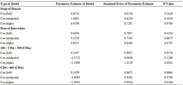
Table 3. Aids data: Effect of stage of disease and dose of zidovudine.

curred.
Interval-censored data often occur in medical applications. As seen in the AIDS data set, when data are heavily censored, making assumptions about when events occurred and using techniques such as Cox regression can lead to inaccurate conclusions. It can also result in unstable estimation in the non-parametric methods. The parametric methods available in SAS, S-Plus and R are the most readily available alternatives. As seen with the examples presented in this paper, these parametric approaches can be highly satisfactory in their performance. This is especially so if one chooses the Weibull or lognormal family that allows a reasonably wide range of distributional shapes.
Results using the Cox regression models, the exponential, Weibull and log-normal models for the Hemophilia data are shown in Table 4. Parameter estimates of each of the above models considered, standard errors and Pvalues obtained for these different models are presented in this Table. All of these four analyses show significant evidence of treatment effects.
4. Conclusions and Further Work
Interval censoring has become increasingly common in the areas that produce failure time data. This type of data frequently comes from tests or situations where the objects of interests are not constantly monitored. Thus events are known only to have occurred within particular time durations. The purpose of this study was to illustrate available parametric and non-parametric methods that consider the data as being interval censored.
The time to event ignoring the effects of covariates has been considered using five different techniques. The Kaplan-Meier estimator is used, assuming the event occurred at the left interval, or at the right interval. A Weibull model, where the survival function is modeled using the estimates from SAS PROC LIFEREG is carried out. A Third approach is accomplished by modeling the interval-censored nature of the data using the methods proposed by Turnbull [8]. Splines models presented by Kooperberg and Stone [18] are implemented. Finally, the survival function is estimated using the piecewise exponential model. Parametric models for interval-censored data can follow a number of distributions such as generalized gamma, the log-normal, the Weibull and the exponential distribution. Different independent covariates or categorical variables have also been included in the model to study their effect on the response variable.
Parametric and non-parametric methods of analysis are two different types of techniques in general for the analysis of censored data. However, for the analysis of interval-censored data, the terminology behind them is the same. An important advantage of parametric inference approaches is that their implementation is quite straightforward in principle and the theory of standard maximum likelihood can be applied. A primary disadvantage of these methods is that there often does not exist enough prior information or data to verify a parametric model. The major advantage of non-parametric methods such as Kaplan-Meier and Turnbull approach is that, one can avoid complicated interval censoring issues and make use of the existing inference procedures for the rightcensored data. It is also assumed that the censoring mechanism or variables are independent of the survival variables of interest.
For the Breast Cancer example, the Kaplan-Meier estimates, bracket the Turnbull estimate. The Turnbull curve lies very close to both Weibull and logspline curves. At the same time, Weibull estimates and logspline estimates are quite close to each other. Cox regression models and parametric models with covariates using Exponential, Weibull and Lognormal were fitted. Four analyses produced similar results qualitatively and all showed an increased hazard for group on radiation and chemotherapy which was statistically significant.
Unlike the results obtained for the Breast Cancer data, the estimated survival curve for AIDS data took very few steps in the non-parametric models. Possible explanations could be that the sample size is small, and the observed information was very limited due to interval cen
Table 4. Hemophilia data: Effect of treatment on time to event.

soring. The Kaplan-Meier estimates no longer bracketed the Turnbull estimate. The logspline estimate tracks the parametric models closely. The non-parametric methods were not very helpful in understanding the AIDS data. For the covariate effects of time to development of resistance, stage and dose were taken into account. All methods indicated an increased risk of developing resistance for the patients in a later stage of disease. The Cox model results were highly dependent on the assumptions about when the event occurred. No methods showed a significant effect of dose on the time to development of resistance.
The estimated survival curve for the AIDS data took very few steps in the non-parametric models, which reflected the high degree of censoring in this small data set. For the AIDS data, we took a look at the individual effects of stage and dose on the time to development of resistance. For these data, the non-parametric methods were not very helpful in understanding this data. For the breast cancer data, the four analyses gave similar results qualitatively. All showed an increased hazard for the group on radiation and chemotherapy which was statistically significant. Kaplan-Meier estimates, as expected, bracket all other survival curves.
For the Hemophilia data, the results derived were very much similar to those of Breast Cancer and AIDS data sets except the logspline model. Cox regression models and parametric models with covariates using Exponential, Weibull and Lognormal were fitted. Four analyses produced similar results qualitatively and all have shown an increased hazard for the group on radiation and chemotherapy, which is statistically significant. Results derived for the piecewise exponential are not accurate for all three data sets.
Major statistical packages such as SAS, S-Plus and R have procedures for analyzing interval-censored data using parametric models. Some non-parametric methods are easily programmed. In particular, the Turnbull [8] method for non-parametric estimation of the survival distribution, the Kooperburg and Stone [18] logspline estimates of the survival function and Finkelstein’s (1986) test for covariates are recommended. As seen in the AIDS data set, when data are heavily censored, making assumptions about when events occurred and using techniques such as Cox regression can lead to inaccurate conclusions. It can also result in unstable estimation in the non-parametric methods.
As examples presented in this paper show, parametric approaches can be highly satisfactory in their performance. Especially when the Weibull or log-normal family is chosen, it allows a reasonably wide range of distributional shapes. To allow more flexible modeling with weak parametric assumptions, we suggest the use of a piecewise constant hazards model. Finkelstein and Wolfe [3], Self and Grossman [21], Miller [22] and Buckley and James [23] have all proposed tests for assessing the covariate effects.
NOTES
#The first draft of the paper was completed while this author was at the University of Guelph, Guelph, Canada, and the second author was a grad-student there.
†Corresponding author.