1. Introduction
W.-Y. Hsiang [1] investigated the rotation hypersurfaces of constant mean curvature in the hyperbolic or spherical  -space. In [2], Eells and Ratto have constructed the rotation (
 -equivariant) minimal hypersurfaces in the unit 3-sphere with standard metric by using a certain first integral, which is invariant with respect to the rotation angle of generating curves on the orbit space. In [3], a family of
  -equivariant periodic CMC surfaces was constructed in the Berger spheres when the constant mean curvature (CMC) is a sufficiently small positive number, and it was cleared that the conserved quantity can be obtained by using the Lagrangian equipped with suitable potential function of the corresponding dynamical system with respect to the Hsiang-Lawson metric [1,4] on the orbit space via the Hamilton equation, where the rotation angle of generating curves can be regarded as “time”. We should remark that the corresponding Lagrangian has the vanishing potential when we construct the
  -equivariant minimal hypersurfaces. However, in case that we construct the
  -equivariant non-minimal CMC-hypersurface in the Berger sphere, the potential of the Lagrangian is a nonvanishing function. In Theorem 4.3, we determine the potential function of the Lagrangian which corresponds to the
  -equivariant CMCsurfaces immersed in the Berger sphere. As a result we can obtain a family of periodic
  -equivariant CMC surfaces in the Berger spheres when the constant mean curvature is an arbitrary positive number (Theorem 5.2).
2. Preliminaries
In [3], a generalized inner product  on the unit 3- sphere
  was defined by

where ,
, and
and  ,
,  and
and  are positive and nonnegative parameters, respectively. The Cartan hypersurface
  in the unit 4-sphere is covered by
  (via an 8-fold covering), whose metric is rescaled along the Hopf fibres and its metric on
  coincides with
  [5,6]. The family of metrics
  defined on
  contains this one as a special case. In particular
  is a left-invariant metric on
  and
and  is called the Berger sphere with metric
  in case that
 . The Berger metrics
  are obtained from the canonical metric by multiplying the metric along the Hopf fiber by
  [7].
[7].
Throughout the paper we consider the Berger spheres . Here we summarize the notations which are used in the paper.
 denotes the orbit space by
  -isometric
  - ction
  as follows.

As the parametrization of  we use the following map:
 stands for the orbital metric on
  :
:

 is the volume function of orbits and
  is the Hsiang-Lawson metric on
 :
:

where

 denotes a curve parametrized by arclength
 . And also
  and
and  stand for the tension fields of
  with respect to the metrics
  and
and , respectively. The geodesic curvature
  at
at  is defined by
  where
where  denotes the unit normal vector field to
 .
.
3. S1-Equivariant CMC-Immersion
For a curve , we consider an
  -equivariant map
  such that
  , where
  and
and  are Riemannian submersions. Throughout the paper, we assume that
  is an
is an  -equivariant constant mean curvature
  immersion. Then we have
 (1)
(1)
since

On the orbit space , the velocity vector field of a curve
  is given by the following component functions.
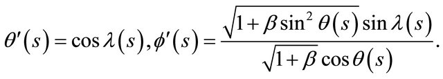
Lemma 3.1. The following formulas hold on  .
.
 (2)
(2)
 (3)
(3)
where
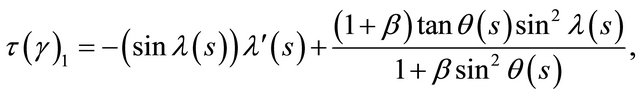
and

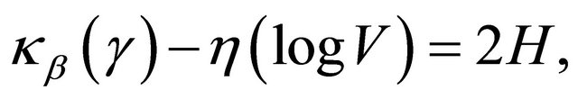
Then using the formula (1) we have the following differential Equation (4) of generating curves which corresponds to the CMC-rotation hypersurfaces immersed in , since using Lemma 3.1 the geodesic curvature
  is given by
 (4)
(4)
4. Conservation Laws
We consider a generating curve  on
on  such that
  and
and . Then we can consider the space
  of motion with
and time . Let
. Let  be a Lagrangian on
 . Via the Legendre transformation we have the Hamiltonian
  on the phase space
 :
:

The conservation laws of our system imply the following Proposition 4.1. Let the Lagrangian  on
on  be the following form:
 where
where  is the Hsiang-Lawson metric on
  and
and  is a potential function on the configuration space.
Then we have
 (5)
(5)
where the conserved quantity in the formula represents the Hamiltonian of our system.
By means of the Hamilton equation (5), we shall determine the potential  which corresponds to the
  -equivariant CMC surfaces immersed in
  via the differential Equation (4) of generating curves on the orbit space
 .
.
The direct computation yields the following Lemma 4.2. Assume that  and
and  are functions of
 and
and . Then we have
 (6)
(6)
where

As a consequence, we have the following Theorem 4.3. On our system, the Lagrangian  and the Hamiltonian
  which correspond to the
  -equivariant CMC-H hypersurface immersed in
  can be determined as follows:

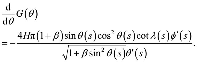
Proof. Using Lemma 4.2 and the differential equation of generating curves (4) we have

from which we obtain
Since  is a constant mean curvature and
we can choose such as . Q.E.D.
5. Generating Curves for S1-Equivariant CMC Surfaces
Let  be a generating curve on
  such that
  and
and  with the arc length
 . Then we set the following initial conditions:

The Hamilton equation  (Theorem 4.3) implies that

from which we have

where

On the other hand, using the formulas

and

we have

Consequently we have the following Lemma 5.1. Under the initial conditions for generating curves which correspond to the CMC-H rotation hypersurfaces, we have

and
 (resp.,
 ) if and only if,

where

Assume that  is an arbitrary positive number. In Lemma 5.1 we now choose
  such that
 .
.
From Lemma 5.1,  and there exists the value
  of
of  such that
  decreases strictly until
 , where the value of
  equals to zero at
 , and
, and  takes a local minimum at
 . In fact, if
  does not take a local minimum, then we may assume that there exists
such that  and
and
 .
.
Then from the differential equation (4) of generating curves it follows that . On the other hand we obtain the following formula:
 (7)
(7)
where

The formula (7) implies that
 (8)
(8)
where

The formula  implies that

from which we have

since .
.
Hence we see that is a positive number. Now if
 , then
 , which implies that
  and
and
 , hence
 , which is a contradiction. Therefore, the value
  is not zero.
Consequently, since , from the formula (8)
we see that  is not zero, which contradicts the assumption
 . Hence
takes a local minimum.
Thus we can continue as the curve satisfying the differential Equation (4) by the reflection. Let
  be the right hand side of (7). We can define
  by
by  as follows:

Consequently we have the following Theorem 5.2. Let  be an arbitrary positive number and choose
  such that
 . If
. If  is a rational number, then the corresponding
  -equivariant hypersurface is an immersed CMC-H torus in the Berger sphere
 . In particular, if
  is an integer, then this CMC-H torus is embedded.
Theorem 5.3. In the case , Then the corresponding
  -equivariant CMC-H hypersurface in the Berger sphere
  is an extended Clifford torus

where

Corollary 5.4. There exists an embedded minimal torus in the Berger sphere 

6. Acknowledgements
I am grateful to Yoshihiro Ohnita and Junichi Inoguchi for their encouragement.