1. Introduction
Toroidal functions have been known for a long time and an important bibliography is given in [1,2] with some applications to diffraction of acoustic and electromagntic plane waves by a torus. These functions have played a major role in the analysis of plasma confinement in a torus configuration [3], where further references can be found] and, more recently, important works have been devoted to their application in particular situations [4-6].
We are interested here in TE, TM electromagnetic fields in a toroidal medium which becomes of importance for the so-called transformation media: a tool used to tackle invisibility problems [7]. We start with a presentation of the main properties of the toroidal coordinates x, q, f. Then, we discuss the Maxwell equations satisfied by the components Ef, Hx, Hq of TE modes (it is easy to transpose these results to TM modes Hf, Ex, Eq) and, we finally get the wave equation satisfied by Ef. Approximate solutions of this equation are obtained when the index of refraction in the toroidal space makes separable the wave equation.
2. Toroidal Coordinates
2.1. Geometric Parameters
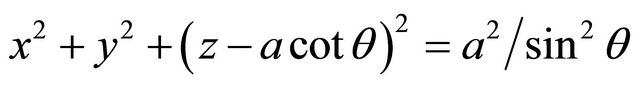
In terms of the Cartesian coordinates x, y, z, the toroidal coordinates  ,
,  ,
,  are defined by the relations [8-10]
 (1)
(1)
in which  with the inverse relations
 (2)
(2)
 (2a)
(2a)
The surfaces of constant  correspond to spheres with different radii
 (3a)
(3a)
the surfaces of constant x are non intersecting tori of different radii (anchor rings)
 (3b)
(3b)
the normal derivative to these surfaces is
 (4)
(4)
Now, from the toroidal metric

 (5)
(5)
we get the scale functions
 (6)
(6)
so that the volume element is
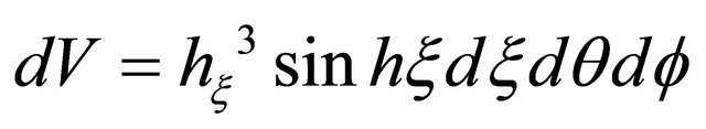 (7a)
(7a)
and the surface elements
 (7b)
(7b)
Remark: the metric (5) may be written with (i,j) = 1, 2, 3 and summation on the repeated indices

 and,
and,  denoting the matrix with components
 , it comes g = diag. a2h2 (1, 1, sinh2x) where
 .
.
2.2. Differential Operators
Using the general definition of the differential operators in orthogonal coordinates [10,11], we get gradient:
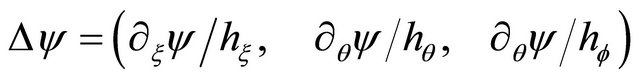 (8a)
(8a)
divergence:
 (8b)
(8b)
curl:
 (8c)
(8c)
and, for the laplacian of a scalar field
 (9)
(9)
3. TE Field
The components of the TE field  are not function of the
  coordinate and, using (8c), it is easy to get, in a homogeneous isotropic medium with permittivity
  and permeability
  the Maxwell equations they satisfy
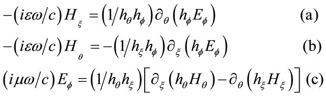 (10)
(10)
Substituting (10(a) and (b)) into (10(c)) gives the wave equation satisfied by 
 (11)
(11)
Multiplying (11) by  and using (6(a)), we get with
 (11a)
(11a)
 (12)
(12)
and, since 
 , this equation becomes
 (13)
(13)
To get a more tractable wave equation, we introduce [8,10] fhe variables  and the function
 ,
,
 (14)
(14)
and we write (13) A + B + C = 0.
Then, the expression (6(b)) of  is written with the parameter a deleted
 (15a)
(15a)
and  is changed into
  implying
 (15b)
(15b)
so that
 (16)
(16)
Then, taking into account (14), (15b), (16), the first term  of (13) becomes
 (17)
(17)
and a simple calculation gives since the  terms cancel
 (17a)
(17a)
Similarly with
 (18)
(18)
the second term of (13) becomes
 (19)
(19)
and, a simple calculation gives since the terms  cancel
 (19a)
(19a)
Taking into account (17a) and (19a), we get
 (20)
(20)
 (20a)
(20a)
which reduces as easy to prove to the simple expression
 (21)
(21)
Now, using (14) and the expression  of
of the last term
  of (13) becomes
 (22)
(22)
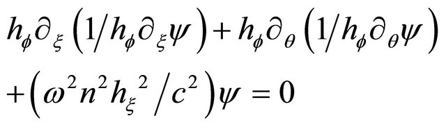
So, according to (20) (20a), (21), (22), the equation (13)  takes the simple form justifying the choice of the function (14) made in [8,10] where calculations for A, B are also made
 (23)
(23)
Deleting the last term in Equation (23) reduces the wave equation to the Laplace equation with the variables  separated so that looking for
  in the form where m is an integer
 (24)
(24)
gives since 
 (25)
(25)
with as elementary solutions [8,10] of this Laplace equation, the half order Legendre functions  of first and second kind.
Now, the wave  (23) for TE fields may be generalized to a medium with a constant permitivity while the permeability, consequently the refractive index, depends on
  and
and . So, to make
  (23) separable, we assume that the refractive index n is with
  constant
 (26)
(26)
Then, the last term of (23) becomes  where
where  and with
 (27)
(27)
in which m is no more assumed to be an integer, the wave equation satisfied by  is
is
 (28)
(28)
and with  we get
 (29)
(29)
whose solutions are the conical (Mehler) harmonics [10, 12] 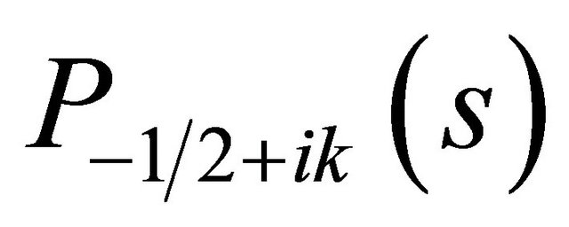 and
and .
.
Then, according to (11a), (14), (27), the component  of the TE field is
 (30)
(30)
in which  and
and 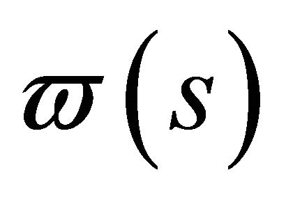 solution of (23). Substituting (30) into (10(a) and (b)) gives the magnetic components
 of the TE field.
TM field: These results are easy to transpose to TM fields: just change , and
, and  .
.  into
into  and
and  .
.  with a constant permeability while the permittivity is defined so that the refractive index has still the expression (26).
4. Discussion
This work is an illustration of the importance of the function (14) in toroidal coordinates either as in [8,10] to make manageable the 3D Laplace equation which separates into three equations. or as here to get a similar result with the 2D Helmholtz equation. It is remarkable that for TE, TM propagation in a toroidal medium this choice of a particular form for the  component of these fields works so efficiently that we get an exact equation whatever is the refractive index. In some sense, the function (14) is consubstantial to toroidal and bispherical coordinates.
The results obtained here are only illutrative because to get analytical solutions of the exact Equation (23), satisfied by , we had to impose rather drastic conditions on the refractive index with a constant permittivity (TE) or constant permeability (TM) , in order to get a separable equation. In practice, to solve (23), requires numerical calculations with algorithms to tackle 2D partial differential equations which is not a real difficulty in particular for propagation in isotropic homogeneous media where the refractive index is constant.
The toroidal geometry has made a comeback in two different domains: first in the string theory of elementary particles [13,14] and second in cosmology. The quest of cosmic origin [15] has suggested [16] that the Universe could have the shape of a drough nut that is of a 3D torus.
Clearly, the present work on electromagnetic wave propagation in a toroidal space could be of some interest to toroidal cosmology [17-19].