Ductile Fracture Characterization for Medium Carbon Steel Using Continuum Damage Mechanics ()
1. Introduction
Ductile fracture is the failure of a solid material due to nucleation, coalescence and growth of cavities induced by plastic deformation. There are several ways, from empiric relationships [1,2] to porous media stiffness modeling [3], developed to study this phenomenon in order to predict when a workpiece will fail under a given stressstrain state.
Kachanov, in 1958 [4], first proposed a continuum damage variable to represent the surface density of cavities in a given infinitesimal volume element. By the 70’s, researchers embraced the idea and developed a theory based on the framework of irreversible processes thermodynamics to model the evolution of this damage variable and how it affects mechanical properties, such as elastic modulus and stresses, leading to the eventual failure of a material [5]. This theory, called Continuum Damage Mechanics (CDM), is complementary to Fracture Mechanics, since it is concerned about the nucleation and growth of cavities until they reach a critical size turning into a macroscopic crack, whose propagation in a solid media is studied by the latter.
For damage evolution caused by large plastic deformation, Lemaitre and Chaboche developed the first and simplest model [6-10], which considers a linear evolution of isotropic damage with plastic strain in a uniaxial stress state condition. This model was later expanded by other authors, adding new capabilities such as dealing with anisotropic damage [11], or with non-linear damage evolution [12-16].
Recently, medium carbon steel heat-treated to obtain spheroidized cementite in its microstructure is being used as raw material for sheet forming processes, due to its better formability properties [17]. Due to large plastic strains imposed to this kind of manufactured parts, cracks and other defects observed are mostly related to ductile damage evolution.
With this motivation, in this work the ductile fracture of SAE 1050 steel was studied, for two different microstructural conditions namely: lamellar ferrite-pearlite and spheroidized cementite, under the continuum damage mechanics point of view. Experimental characterization of isotropic damage evolution was carried out and numerical simulations were performed in order to predict failure.
2. Continuum Damage Mechanics Model for Ductile Fracture
The continuum damage variable introduced by Kachanov is defined as the relationship between the sectional area of voids  and the overall sectional area
  of a given surface in a volume element. Assuming the hypothesis of isotropic deterioration of the material, the damage can be written as:
 (1)
(1)
where  is the effective resisting area. It may be observed that this definition is the same one as the microvoid area fraction used is some micromechanical theories, such as McClintock’s [18]. The damage variable can assume any value between 0 and 1, covering from a virgin state to a completely damaged one, although real materials will fail when the damage reaches a critical value
 , when the effective area can no longer resist the applied load, leading to the formation of a macroscopic crack.
In his model, Lemaitre assumes the hypothesis of strain equivalence, which states that the damaged material will have the same constitutive behavior of the virgin material, replacing the stress tensor  by the effective stress tensor
 , defined as:
 (2)
(2)
One important consequence of this assumption is that one can define an effective elastic modulus of a damaged material, giving an indirect way to measure the damage in a solid, by monitoring the evolution of the Young modulus with increasing strain:
 (3)
(3)
where  is the effective elastic modulus and
  is the elastic modulus for the undamaged material.
Using as basis the thermodynamic of irreversible processes [19], CDM treats the damage as an internal thermodynamic state variable, and so its evolution can be derived assuming the existence of a potential of dissipation  and an associated variable Y, named damage strain energy release rate and defined as [10]:
 (4)
(4)
where  is the von Mises equivalent stress,
  is the deviatoric stress tensor,
  is the Poisson’s ratio and
  is the hydrostatic stress. Further, Lemaitre [10] shows that the damage evolution can be written as:
 (5)
(5)
with  defined as the accumulated plastic strain and
  being the plastic strain tensor. The choice of a proper potential of dissipation that can represent experimental results is the core of any CDM model. In Lemaitre and Chaboche’s model, the hypothesis of isotropic damage, existence of a strain threshold for damage initiation and linear evolution of the damage with the accumulated plastic strain leads to the following equation for damage evolution:
 (6)
(6)
where  is the accumulated plastic strain threshold and S is the damage resistance parameter, which are material dependent properties. For the uniaxial stress state, and assuming that the elastic strain can be neglected in comparison to the total strain, the accumulated plastic strain can be considered equal to the principal strain. The damage increases until it reaches a critical value
  which can be calculated with the following equation [10]:
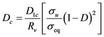 (7)
(7)
where  is the critical damage for the uniaxial stress state and can be measured in a tensile test,
  is the ultimate tensile stress and
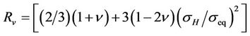
is called triaxiality factor, which accounts for the difference between the actual stress state and the perfectly uniaxial stress state.
This model was later implemented in the Abaqus/Explicit solver using the VUMAT subroutine [20] following the numerical algorithm proposed by Lee and Pourboghrat [21].
3. Experimental Procedure
In order to determine mechanical properties and damage parameters, standard tensile tests were carried out for specimens of SAE 1050 steel for the lamellar and for the spheroidized microstructures. Three specimens for the hot rolled ferrite-pearlite material and nine specimens for the spheroidized material were tested.
The spheroidized material has been cold rolled, with a thickness reduction of 50% and subsequently annealed at 700˚C for 13 hours in a 100% H2 atmosphere, to obtain the characteristic spheroidized microstructure. The specimens were machined from a 1.0 mm thickness sheet (spheroidized material) and from a 2.0 mm thickness sheet (hot rolled material. The neck section had 75 mm length and 12.5 mm width, as shown in Figure 1.

Figure 1. Workpiece dimensions, in mm, for the tensile test.
The damage variables were calculated using the variation of the elastic modulus, so several loading-unloading cycles were needed in order to measure this property with strain increase. The tests were performed in an Instron 3369 universal testing machine, with a 50 kN load cell. Each cycle began with a 1 mm crosshead displacement followed by an unloading until the force attained 50 N. The crosshead velocity was fixed at 2 mm/min. The strains were measured through a clip gage extensometer with 50 mm gage length. Sampling frequency was 5 Hz. Figure 2 illustrates the experimental setup.
Figure 3 shows the true stress-strain curves for both types of tested specimens. The loading-unloading cycles shown were used in the evaluation of the elastic modulus, measured always during the unloading path, following recommendations by Lemaitre [10]. The drop in the true stress, as pictured in this figure, can be linked to the fracture initiation. To represent the work hardening behavior of the material, Ludwik equation [22] has been used, as presented by Equation (8). The material constants are given in Table 1.
 (8)
(8)
The evolution of the elastic modulus is shown in Figure 4 for the tested materials (including the pure iron results [23] and other carbon steels [24,25] obtained from the literature). It may be observed that the elastic modulus decreases with increasing carbon level. Also, there is a significant non-linear drop in the elastic modulus for small strains, followed by a linear evolution. Lemaitre’s model considers that the damage does not occur for a strain below the critical value, and will grow with a constant rate after that value. For this reason, following the same procedure of Celentano et al. [24], any elastic modulus degradation below the linear part of the curve will be neglected. This transition coincides with the transition of the elastic regime to the plastic behavior of the material. Therefore, yielding strain will be considered as the damage strain threshold and the elastic modulus, at this point, will be assumed to be the one for the undamaged material.
The damage evolution, measured trough Equation (3), is shown in Figure 5 for both studied alloys. Critical damage  is taken as the damage value prior to the non-linear increase in damage, just before fracture. The
 (a)
(a) (b)
(b)
Figure 2. Experimental setup for the tensile tests.
other parameter to be evaluated is the damage resistance S, calculated trough Equation (9), which is obtained by manipulating Equation (6) and assuming that in the tensile test the material is under a perfectly uniaxial stress state.
 (9)
(9)
To obtain the value of S, several experimental points must be taken from Figures 3 and 5 for different strains.
Table 1 summarizes the mechanical and damage parameters identified for SAE 1050 steel for both microstructural conditions.
It must be pointed out that these parameters can be used as inputs for finite element simulations of the tensile test.
4. Numerical Simulations
Lemaitre’s model was implemented in Abaqus/Explicit finite element solver using a VUMAT subroutine aiming at the coupling of isotropic plasticity with damage, based on the stress integration algorithm called operator-split.
For each time step, the incremental strain was considered as being fully elastic, and then the corresponding stress tensor was evaluated. The von Mises criterion, coupled with damage, was used to determine if the material is indeed below the yielding condition:
 (9)
(9)
If Equation (10) is not satisfied, then a plastic correcting procedure must be used to calculate the plastic increment and ensure the consistency condition. Details of this plastic corrector can be found in Lee and Pourboghrat [22]. After this calculation, stresses, the damage variable and the plastic strain are updated for the next step. Further details may be obtained in Tsiloufas [26].
The tensile test was simulated using an imposed longitudinal displacement on the right end of the specimen, with the same 2 mm/min velocity as for the experimental procedure. Boundary conditions of restricted transversal
 (a)
(a) (b)
(b)
Figure 3. True stress-strain curves for SAE 1050 steel. (a) Spheroidized alloy, (b) Hot rolled alloy.
and normal displacement were imposed for both ends of the specimen, simulating the jaws of the tensile test equipment. The mesh in the test region is formed by 4500 solid hexahedral elements, with 8 nodes, linear integration and 0.5 mm length.
Figure 6 shows the resulting true stress-strain curves. The numerical simulations could properly reproduce the work hardening behavior of the tested materials, however the difference between the effective stress  , that is measured through the load cell