1. Introduction
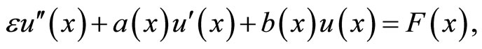
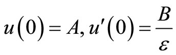
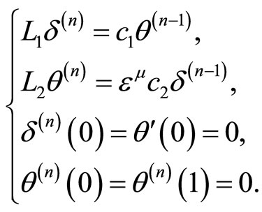
We consider the following singularly perturbed initial/ boundary value problem for the linear system of ordinary differential equations in the interval :
:
 (1)
(1)
 (2)
(2)
 (3)
(3)
 (4)
(4)
where  is a small parameter
 A1, A2, B1, B2, are given constants. The functions


 are given functions satisfying certain regularity conditions which are specified whenever necessary.
The above type initial/boundary value problems arise in many areas of mechanics and physics [1,2].
Differential equations with a small parameter  multiplying the highest order derivative terms are said to be singularly perturbed and normally boundary layers occur in their solutions. The numerical analysis of singular perturbation cases has always been far from trivial because of the boundary layer behavior of the solution. Such problems undergo rapid changes within very thin layers near the boundary or inside the problem domain. It is well known that standard numerical methods for solving such problems are unstable and fail to give accurate results when the perturbation parameter
  is small. Therefore, it is important to develop suitable numerical methods to these problems, whose accuracy does not depend on the parameter value
 , i.e. methods that are
  -uniformly convergent. These include fitted finite difference methods, finite element methods using special elements such as exponential elements, and methods which use a priori refined or special non-uniform grids which condense in the boundary layers in a special manner. The various approaches to the design and analysis of appropriate numerical methods for singularly perturbed differential equations can be found in [3-8] (see also references cited in them).
In this present paper, we analyze the numerical solution of the initial/boundary problems (1)-(4). The numerical method presented here comprises a fitted difference scheme on an uniform mesh. Fitted operator method is widly used to construct and analyse uniform difference methods, especially for a linear differential problems (see, e.g., [4-7]). In the Section 2, we state some important properties of the exact solution. The derivation of the difference scheme and uniform convergence analysis have been given in Section 3. Uniform convergence is proved in the discrete maximum norm. The approach to the construction of the discrete problem and the error analysis for the approximate solution are similar to those in [8,9].
Difference schemes for singularly perturbed systems with another type of initial/boundary conditions was investigated in [9-14].
Throughout the paper, C will denote a generic positive constant independent of  and of the mesh parameter.
2. Analytical Results
Here we give useful asymptotic estimates of the exact solution of (1.1)-(1.4), that are needed in later sections.
Lemma 2.1 Under the
 (5)
(5)
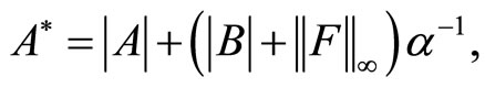
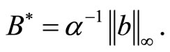
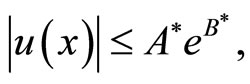
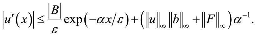
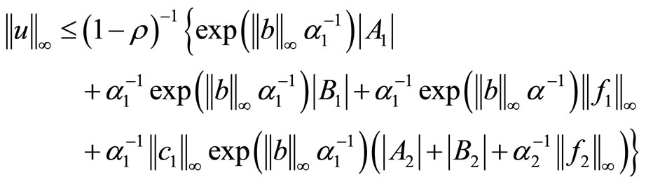
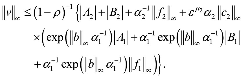
the problem (1.1)-(1.4) has a unique solution, which satisfies
 (6)
(6)
 (7)
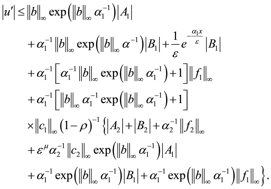
(7)
 (8)
(8)
 (9)
(9)
where  for any continuous function
 .
.
Proof. Consider the iterative process
 (10)
(10)
where  is an arbitrary function.
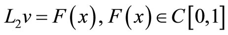
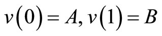
First we prove that for the solution of initial-value problem of the type
the following estimates hold
 (11)
(11)
 (12)
(12)
To prove (2.7), after some manipulations we have
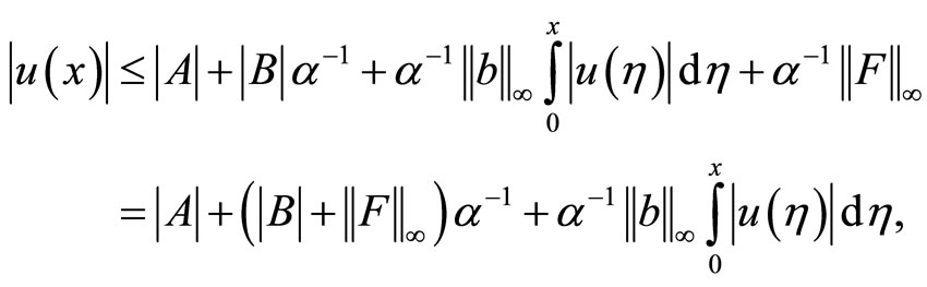
hence
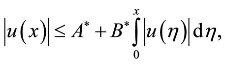
with
From here by virtue of integral inequality it follows that
which leads to (2.7). Now we prove (2.8). Clearly
Then by using (2.7) we get
which arrive at (2.8).
Further, note that, by virtue of maximum principle the problem of the form
admits the estimate
 (13)
(13)
Denoting
from (1.1)-(1.4) and (2.6) we have
Next, applying here (2.7), (2.8), (2.9) we arrive at
Therefore
 (14)
(14)
with
 (15)
(15)
From (2.10) we have
 (16)
(16)
 (17)
(17)
 (18)
(18)
From (2.12), (2.13), (2.14) follows that the sequences  uniformly converges on
for . Replacing (2.6) by appropriate system of integral equations we conclude that for
  the limit functions are the solution of (1.1)-(1.4).
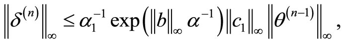
Now the using (2.7) and (2.8) with the function  yield the following stability bounds
 (19)
(19)
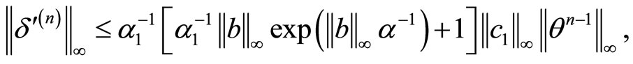
 (20)
(20)
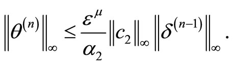
Next from (2.9), with  it follows that
 (21)
(21)
From (2.13) and (2.15) obviously
Using the last relation in (2.14) we obtain
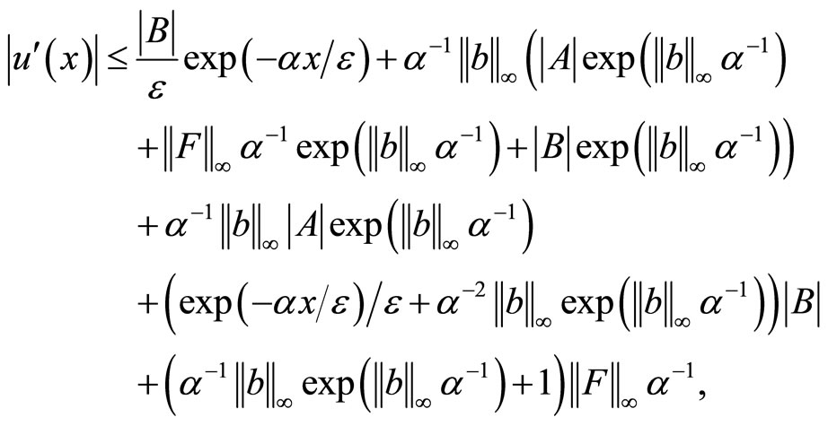
The last three inequalities show the validity of (2.2)- (2.4). Now we prove (2.5). Since
which leads to (2.5), which completes the proof.
3. The Difference Scheme and Convergence
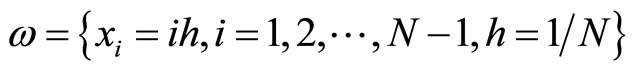
Now we construct the difference scheme and investigate it. In what follows, we denote by  the uniform mesh in
 :
:
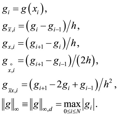
and . Before describing our numerical method, we introduce some notation for the mesh functions. For any mesh function
 , we use
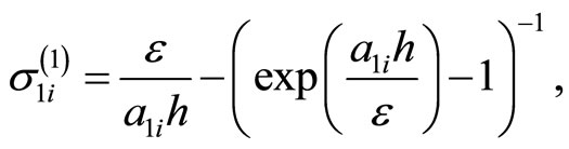
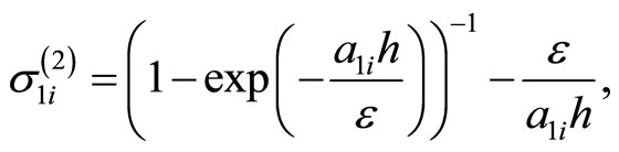
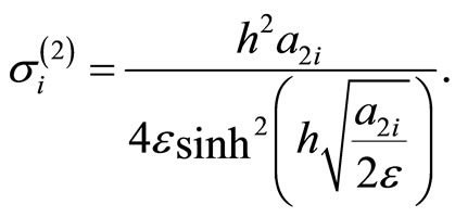
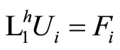
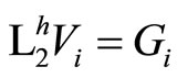
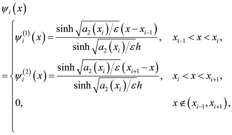
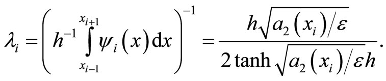
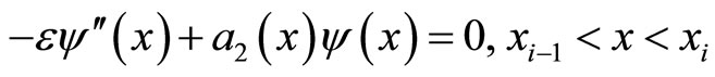
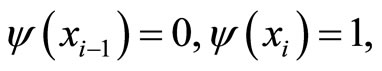
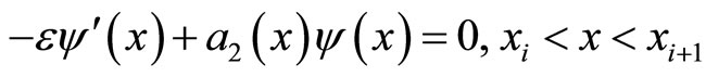
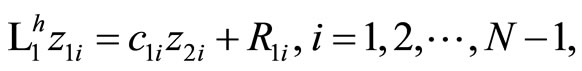
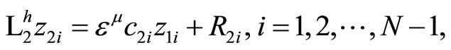
On  we propose the following difference scheme for approximating (1.1)-(1.4):
 (22)
(22)
 (23)
(23)
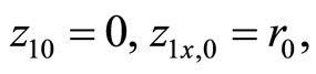
 (24)
(24)
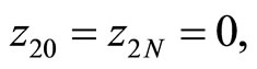
 (25)
(25)
and
For solving of the (3.1)-(3.4) we give the following iterative procedure:
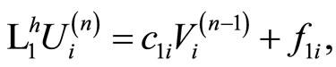

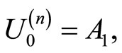
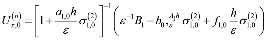

where  is arbitrary.
Lemma 3.1
 (26)
(26)
 (27)
(27)
where  implies the discrete maximum norm on
 ;
;
 and
and  are defined by (2.1) and (2.11) appropriately.
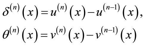
Proof. Denoting 
 we will have
 (28)
(28)
 (29)
(29)
 (30)
(30)
 (31)
(31)
From (3.7)-(3.10), it is not difficult to get
where
and thereby
In similar manner we also obtain
Hence,
Consequently,
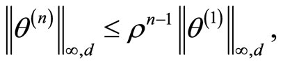
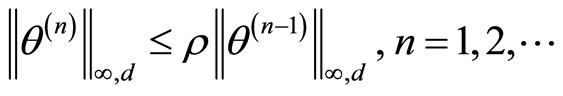
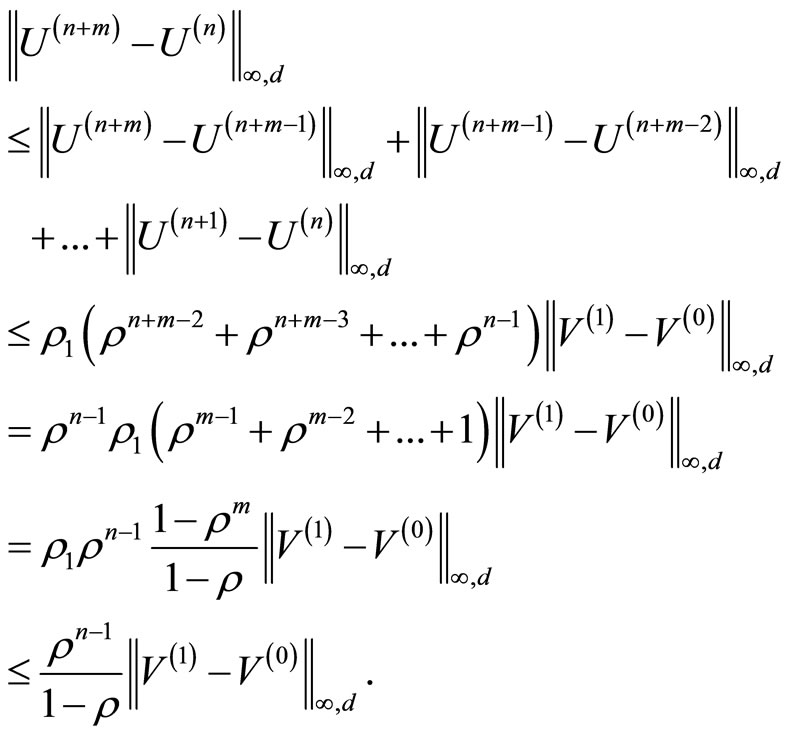
From this follows that the ,
,  to
to , hence the sequences
 ,
,  are the Cauchy sequences and convergent:
  and
and  . The limit functions
 will be solution of scheme (3.1)-(3.4).
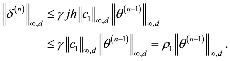
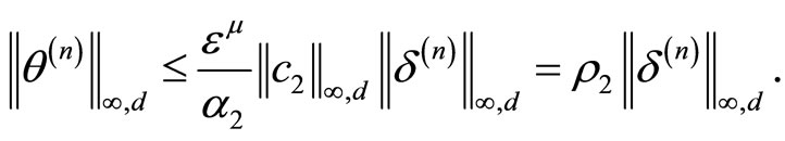
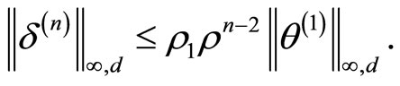
Now we prove (3.5), (3.6). We have
The limit case for  leads to (3.5). The inequality (3.6) is being proved analoguosly.
Lemma 3.2 The solution of the difference problem (3.1)-(3.4) satisfies
 (32)
(32)
 (33)
(33)
where 
 .
.
Proof. Using the estimates for the difference equations
and
with conditions (3.3) and (3.4) appropriately, which is being obtained analoguosly as in differential case, after setting  and
and  we will get
 (34)
(34)
 (35)
(35)
The using each of these into another immediately leads to (3.11) and (3.12).
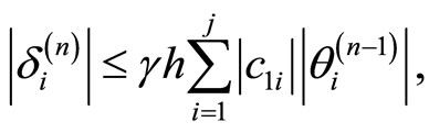
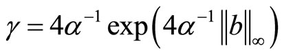
Lemma 3.3 For the truncation errors
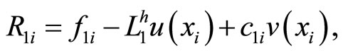
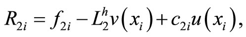
the following estimates hold
 (36)
(36)
 (37)
(37)
 (38)
(38)
Proof. We may write
 (39)
(39)
 (40)
(40)
 (41)
(41)
where
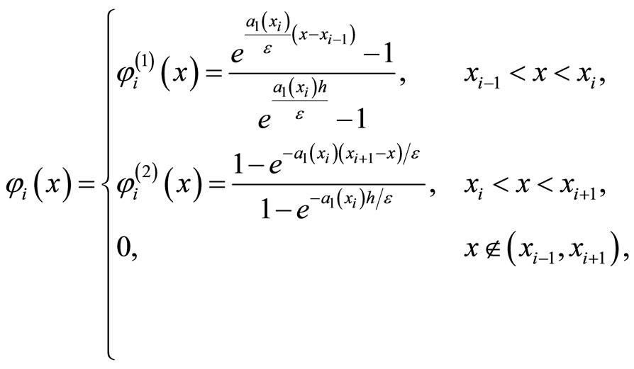
We note that ,
,  and
and ,
,  are the solutions of following problems respectively:
The relations (3.18)-(3.20), by using also the above properties of  and
and  leads immediately to (3.15)-(3.17).
Theorem 3.1 Let 


 Then the solution of the difference problem (3.1)-(3.4) converges uniformly in
  to the solution of (1.1)-(1.4) with rate
 .
.
Proof. Let 
 Then for the errors of the approximate solution
  we have
where  are approximating errors from Lemma 3.3. Using Lemma 3.2, we obtain:
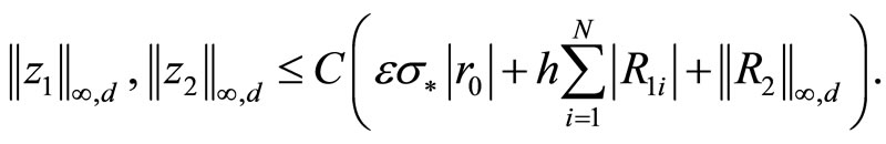
By virtue that of (3.15)-(3.17) all terms in right-hand side of this inequality have the rate  and hence the proof follows immediately.
4. Numerical Example
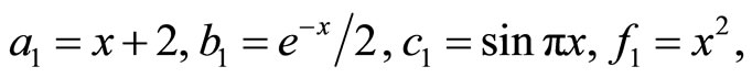
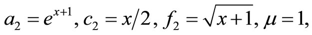
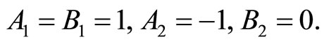
Consider the particular problem with
The initial guess is chosen as
and stopping criterion is
We calculate an experimental rates of convergence  using double mesh method as follows [4,5]:
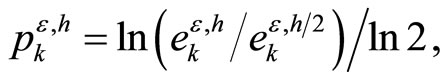
where
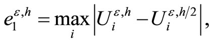
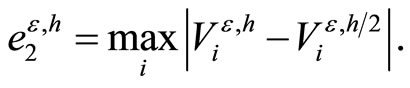
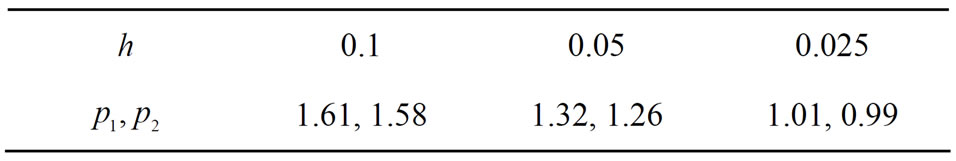
The convergence is uniform, i.e., rate of convergence independenty of perturbation parameter. Some obtained values for
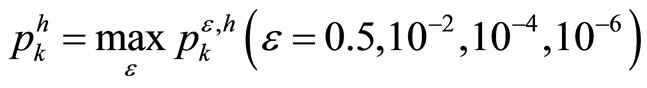
are listed in the table
5. Conclusion
The singularly perturbed initial-boundary value problem for a linear second order differential system is considered. To solve this problem, an exponentially fitted difference scheme on a uniform mesh is presented. First order convergence in the discrete maximum norm, independently of the perturbation parameter is obtained. Obtained in numerical example experimental rates of convergence in agreement with theoretical values.
6. Acknowledgements
The author is grateful to the anonymous referees for his comments and suggestions which helped improve the quality of manuscript.