Numerical Solution of the Fredholme-Volterra Integral Equation by the Sinc Function ()
1. Introduction
In recent years, many different methods have been used to approximate the solution of the Fredholme-Volterra Integral Equations, such as [1,2]. In this paper, we first present the Sinc Function and their properties. Then we consider the Fredholme-Volterra Integral Equation types in the forms
 (1.1)
(1.1)
where ,
,  and f(x) are known functions, but u(x) is an unknown function. Then we use the Sinc Function and convert the problem to a system of linear equations.
2. Sinc Function Properties
The sinc function properties are discussed thoroughly in [3-10]. The sinc function is defined on the real line by
 (2.1)
(2.1)
For , and
, and  The translated sinc functions with evenly spaced nodes are given by
 (2.2)
(2.2)
The sinc function form for the interpolating point  is given by
 (2.3)
(2.3)
Let
 (2.4)
(2.4)
If a function  is defined on the real axis, then for h > 0 the series
 (2.5)
(2.5)
called whittaker cardinal expansion of , whenever this series converges. The properties of the whittaker cardinal expansion have been extensively studied in [8].
These properties are derived in the infinite stripe D of the complex wplane, where for ,
,

Approximations can be constructed for infinite, semiinfinite and finite intervals. To construct approximations on the interval [a,b], which is used in this paper, the eyeshaped domain in the z-plane.

Is mapped conformably onto the infinite strip D via

The basis functions on [a,b] are taken to be composite translated sinc functions,
 (2.6)
(2.6)
Thus we may define the inverse images of the real line and of evenly spaced nodes  as
as

and
 (2.7)
(2.7)
We consider the following definitions and theorems in [8-10].
Definition 2.1:
Let  be the set of all analytic functions, for which there exists a constant, C, such that
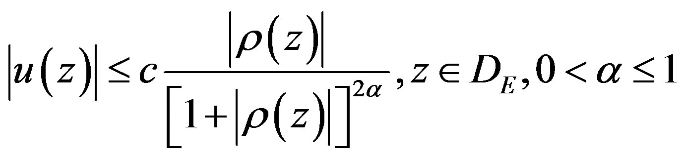 (2.8)
(2.8)
Theorem 2.1:
Let , let N be appositive integer, and let h be
 (2.9)
(2.9)
Then there exists positive constant C1, independent of N, such that
 (2.10)
Proof: See [8,9].
Theorem 2.2:
Let  Let N be a positive integer and let h be selected by the relation (2.9) then there exist positive constant C2, independent of N, such that
 (2.11)
and also for  be defined as in (2.4) then there exists a constant,
  which is independent of N, such that
 (2.12)
Proof: See [8].
3. The Sinc Collocation Method
The solution of linear Fredholm-Volterra integral equation (1.1) is approximated by the following linear combination of the sinc functions and auxiliary functions:
 (3.1)
(3.1)
where
 (3.2)
(3.2)
where the basis functions  defined by
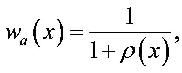 (3.3)
(3.3)
 (3.4)
(3.4)
 (3.5)
(3.5)
We denote then basis function must satisfy the following conditions:
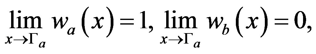 (3.6)
(3.6)
 (3.7)
(3.7)
Obviously by using Equations (2.3) and (3.1) we have

Lemma 3.1:
 , let N be a positive integer and
 , Then (see Equation (3.8)), where
  is defined in (2.14) and C4 is a positive constant, independent of N.
Proof: See [9].
Lemma 3.2:
For  defined in (3.1), let
 and h be selected from (2.9) then (see Equation(3.9))
 (3.8)
(3.8)
 (3.9)
(3.9)
Now let  be the exact solution (1.1) that is approximated by following expansion.
 (3.10)
Upon replacing  in the Fredholm-Volterra integral equation (1.1)
 , applying lemma 3.1 and Lemma 3.2, setting sinc collocation points
  and Then, considering
  we obtain the following system
 (3.11)
We write the above system of equations in the matrix forms:
 (3.12)
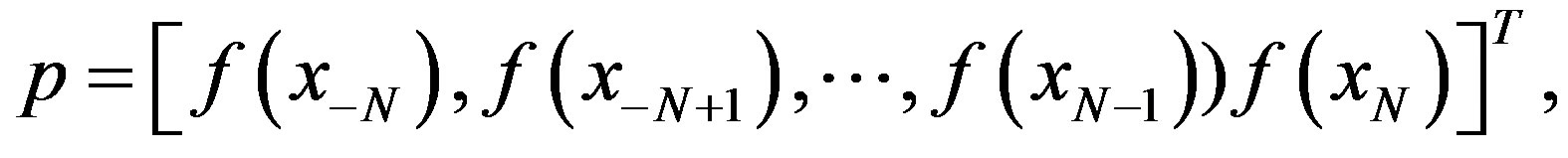
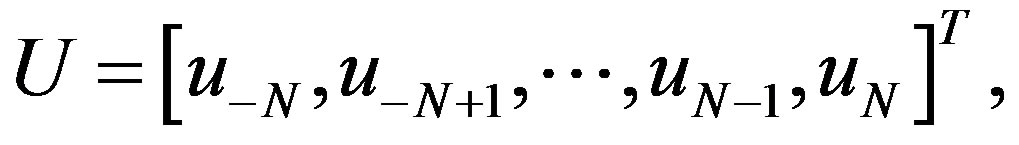
where
 (3.13)
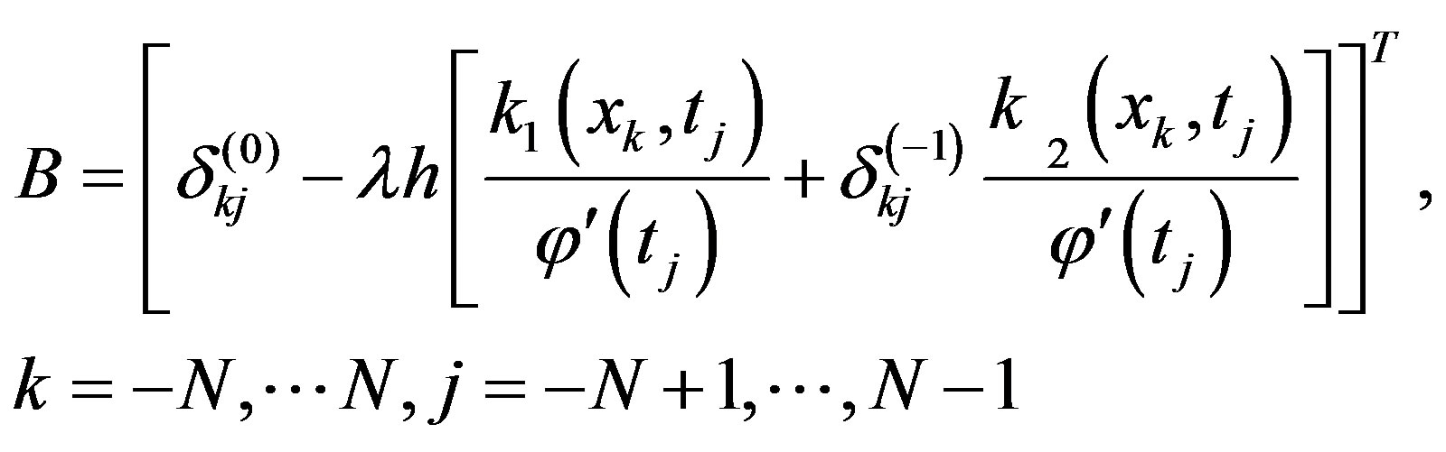 (3.14)
 (3.15)
 (3.16)
 (3.17)
By solving the above system we obtain,  , then, by using such solution we can obtain the approximate solution un as
 (3.18)
4. Convergence Analysis
Now we discuss the convergence each of sinc collocation method. Suppose that  is the exact solution of the Fredholme-Volterra integral equation (1.1). For each N, we can find
  which is our solution of the liner system (3.12), also by using
  we obtain the approximate solution
 , In order to derive a bound for |u(x) - un(x)| we need to estimate the norm of the vector
 , where
  is a vector defined by

where  is the value of the exact solution of integral equation at the sinc points
 . There for we need the following lemma.
Lemma 4.1:
Let u(x) be the exact solution of the integral (1.1) and  let
let

for , then there exists a constant C5 independent of N, such that
 (4.1)
(4.1)
Proof: See [10].
Theorem 4.1:
Let us consider all assumptions of lemma 3.1 and let  be the approximate solution of Fredholme-Volterra integral equation given by (3.3) then we have
 (4.2)
(4.2)
where C6 a constant independent of N, and 
Proof:
Suppose  defined this following form:
 (4.3)
(4.3)

So we have
 (4.4)
(4.4)
By using lemma 3.1, we obtain

Obviously by using equations (4.3) and (3.3) we have.
 (4.5)
(4.5)
And we have from definition of the  We obtain
 (4.6)
(4.6)
That C7 a constant independent of N.
Now, by using equations (4.5) and (4.6) we get
 (4.7)
(4.7)
In this case by using the system (3.12) and lemma 4.1 we obtain
 (4.8)
(4.8)
Now by using Equations (4.7) and (4.8) we get
 (4.9)
(4.9)
Obviously by using Equations (4.9) and (4.2) we obtain

5. Numerical Examples
In this section, we apply the sinc collocation method for solving Fredholm-Volterra integral equation example.
Example 5.1: consider the following Fredholm-Volterra integral equation of the second kind with exact solution u(x) = x.

We solved example 5.1 for different of

And we consider the sinc grid points as:

where

The errors on the given points are denoted by
 (5.1)
(5.1)
Computational results are given in Tables 1-5.

Table 1. Results for Example 1 (N = 5).

Table 2. Results for Example 1 (N = 10).

Table 3. Results for Example 1 (N = 15).
Example 5.2: we consider the following FredholmVolterra integral equation of the second kind with exact solution .
.

Computational results are given in Tables 6-9.

Table 4. Results for Example 1 (N = 20).

Table 6. Results for Example 2 (N = 5).

Table 7. Results for Example 2 (N = 7).

Table 8. Results for Example 2 (N = 9).