Two-Agent Makespan Minimization Problem on Parallel Machines

Siqi Zheng^*, Zhaohui Liu

School of Mathematics, East China University of Science and Technology, Shanghai, China.

DOI: 10.4236/jamp.2023.116110                

Abstract

A two-agent scheduling problem on parallel machines is considered in this paper. Our objective is to minimize the makespan for agent A, subject to an upper bound on the makespan for agent B. In this paper, we provide a new approximation algorithm called CLPT. On the one hand, we compare the performance between the CLPT algorithm and the optimal solution and find that the solution obtained by the CLPT algorithm is very close to the optimal solution. On the other hand, we design different experimental frameworks to compare the CLPT algorithm and the A-LS algorithm for a comprehensive performance evaluation. A large number of numerical simulation results show that the CLPT algorithm outperformed the A-LS algorithm.

Keywords

Parallel Machines, Makespan, Approximation Algorithm, Two-Agent, Empirical Results

1. Introduction

In recent years, management problems in which multiple agents compete on the usage of a common processing resource are receiving increasing attention in different application environments, such as the scheduling of multiple flights of different airlines on a common set of airport runways, berths and material/ people movers (cranes, walkways, etc.) at a port for multiple ships, of clerical works among different “managers” in an office and of a mechanical/electrical workshop for different uses; and in different methodological fields, such as artificial intelligence, decision theory, and operations research.

In this paper, we consider an agent scheduling problem. Unlike classic scheduling problems, the jobs in agent scheduling problem belong to two or more owners which we call agents. Each agent owns a set of jobs and the objective. Each agent has its own goal depending on the schedule of its jobs. All the agents share common resource. Zhao et al. [1] provided an algorithm A-LS with per formance ratio $2-\frac{1}{m}$ . In this paper, we study a two-agent scheduling problem. The two agents are called agent A and B, respectively. All the jobs of agent A and agent B need to be scheduled on identical machines. Our objective is to minimize the makespan for agent A while keeping the makespan for agent B under a given value. The given value is indicated as threshold value for agent B. We only consider feasible threshold value in every instance of the problem, i.e., there always exists a schedule such that the makespan for agent B is no more than the threshold value. According to the notation introduced by Graham et al. [2] , the problem is denoted by $P\mathrm{<mo>\; |\; </mo>\; <mo>\; |\; </mo>}{C}_{\max }^A\mathrm{<mo>\; :\; </mo>}{C}_{\max }^B\le Q$ .

Agent scheduling problems were introduced by Baker et al. [3] and Agnetis et al. [4] . The former paper focused on minimizing a linear combination of the agents’ criteria on single machine and presented some complex results. The latter paper mainly focused on two-agent scheduling problems, they summarized the complexity of some constrained optimization problems. Agnetis et al. [5] extended some of those problems into multi-agent version. Balasubramanian et al. [6] first studied the agent scheduling problem on parallel machines. They established an iteration SPT-LPT-SPT heuristic and a bicriteria genetic algorithm for the two-agent scheduling problem which is $P\mathrm{<mo>\; |\; </mo>}inter\mathrm{<mo>\; |\; </mo>}\left(C_{\max }\mathrm{,}{\displaystyle \sum C^j}\right)$ , where inter means that the jobs of the different sets interfere with one another. Zhao et al. [7] considered two models of two-agent scheduling problem which are $Pm\mathrm{<mo>\; |\; </mo>\; <mo>\; |\; </mo>}{C}_{\max }^A\mathrm{<mo>\; :\; </mo>}{C}_{\max }^B\le Q$ and $Pm\mathrm{<mo>\; |\; </mo>\; <mo>\; |\; </mo>}{\displaystyle \sum C_j^A}\mathrm{<mo>\; :\; </mo>}{C}_{\max }^B\le Q$ , and these two problems had been proved NP-hard. For the problem $Pm\mathrm{<mo>\; |\; </mo>\; <mo>\; |\; </mo>}{C}_{\max }^A\mathrm{<mo>\; :\; </mo>}{C}_{\max }^B\le Q$ , Zhao et al. [1]

provided an algorithm A-LS with performance ratio $2-\frac{1}{m}$ . Moreover, when $m=2$ , they presented an algorithm A-LPTE with performance ratio $\frac{1+\sqrt{17}}{4}\approx 1.28$ . Zhao et al. [8] studied a multi-agent scheduling problem on two identical parallel machines which is $P\mathrm{2\; <mo>\; |\; </mo>}CO\mathrm{<mo>\; |\; </mo>}{C}_{\max }^1\mathrm{,}\cdots \mathrm{,}{C}_{\max }^g$ , where CO denotes the situation where each agent completes to finish its jobs as early as possible. They introduced algorithm MML and proved the performance ratio of algorithm MML is ( $1+\frac{1}{6}\mathrm{,2}+\frac{1}{6}\mathrm{,}\cdots \mathrm{,}g+\frac{1}{6}$ ), which was further shown to be tight. Gu et al. [9] extended the problem into m machines: $Pm\mathrm{<mo>\; |\; </mo>}CO\mathrm{<mo>\; |\; </mo>}{C}_{\max }^1\mathrm{,}\cdots \mathrm{,}{C}_{\max }^g$ . An algorithm LLS was proposed for the problem. They proved the agent’s completion time is at most $i+\left(\frac{1}{3}-\frac{1}{3m}\right)$ times its minimum makespan, where the agent with the i-th smallest $\alpha$ point value is the i-th completed agent.

The rest of this paper is organized as follows. In section 2 we briefly describe an integer programming (IP) model and propose a new algorithm called CLPT. In section 3 we compare the performance between the CLPT algorithm and the optimal solution first and then compare the performance between the A-LS algorithm and the CLPT algorithm. Finally, in section 4 we conclude the paper and give some fruitful directions for future work.

2. Integer Programming Model and the CLPT Algorithm

2.1. Problem Formulation

Agent A has $n_A$ jobs, we denote the job set of agent A by

$J^A=\left\{J_1^A,J_2^A,\cdots ,J_{n_A}^A\right\}$ . Agent B has $n_B$ jobs, we denote the job set of agent B by $J^B=\left\{J_1^B,J_2^B,\cdots ,J_{n_B}^B\right\}$ . Let $n=n_A+n_B$ . The processing time of $J_j^A$ is

$p_j^A$ , $j=1,2,\cdots ,n_A$ and the processing time of $J_j^B$ is $p_j^B$ , $j=1,2,\cdots ,n_B$ . The two agent are competing agents, i.e., $J^A\cap J^B=\varnothing$ , $J=J^A\cup J^B$ . Let $C_{\max }^A\left(\text{CLPT}\right)$ denote the makespan for agent A obtained by the CLPT algorithm, $C_{\max }^B\left(\text{CLPT}\right)$ denotes the makespan for agent B obtained by the CLPT algorithm, $C_{\max }^A\left(\text{LS}\right)$ denotes the makespan for agent A obtained by the A-LS algorithm and $C_{\max }^B\left(\text{LS}\right)$ denotes the makespan for agent B obtained by the A-LS algorithm. Let $\pi$ be the optimal schedule. Let $C_{\max }^A\left(\pi \right)$ denote the optimal makespan for agent A and let $C_{\max }^B\left(\pi \right)$ denote the optimal makespan for agent B.

2.2. An Integer Programming Model for $P\left|\right|C_{max}^A:C_{max}^B\le Q$

In this subsection, we introduce an integer programming (IP) model which can help us obtain the optimal schedule in small-sized instances. Given an arbitrary optimal schedule ${\pi }^{\prime }$ , Zhao et al. [7] has shown that if $C_{\max }^A\left({\pi }^{\prime }\right)\le C_{\max }^B\left({\pi }^{\prime }\right)$ , then ${\pi }^{\prime }$ can be transformed into a new schedule $\pi$ such that A-jobs are all scheduled before B-jobs on each machine without increasing the makespan for agent A or changing the makespan for agent B, vice versa. Obviously, is also an optimal schedule. Let $\pi$ be the optimal schedule considered in the following analysis in this section.

The IP model can be formulated as follows:

$\begin{array}{l}\min C_{\max }^A\\ \text{s}\text{.t}.{\displaystyle \underset{l=1}{\overset{m}{\sum }}}{\displaystyle \underset{i=1}{\overset{n}{\sum }}}{x}_{ij}^l=1,\mathrm{<mtext>\; \hspace{0.17em}\; </mtext>\; <mtext>\; \hspace{0.17em}\; </mtext>}j=1,\cdots ,n\\ {\displaystyle \underset{j=1}{\overset{n}{\sum }}}{x}_{ij}^l\le 1,\mathrm{<mtext>\; \hspace{0.17em}\; </mtext>\; <mtext>\; \hspace{0.17em}\; </mtext>}i=1,\cdots ,n,\mathrm{<mtext>\; \hspace{0.17em}\; </mtext>\; <mtext>\; \hspace{0.17em}\; </mtext>}l=1,\cdots ,m\\ L_l^A={\displaystyle \underset{j\in A}{\sum }}{\displaystyle \underset{i=1}{\overset{n}{\sum }}}{x}_{ij}^l{p}_j,\mathrm{<mtext>\; \hspace{0.17em}\; </mtext>\; <mtext>\; \hspace{0.17em}\; </mtext>}l=1,\cdots ,m\\ L_l^B={\displaystyle \underset{j\in B}{\sum }}{\displaystyle \underset{i=1}{\overset{n}{\sum }}}{x}_{ij}^l{p}_j,\mathrm{<mtext>\; \hspace{0.17em}\; </mtext>\; <mtext>\; \hspace{0.17em}\; </mtext>}l=1,\cdots ,m\end{array}$

$\begin{array}{l}{L}_l={\displaystyle \underset{j\in A\cup B}{\sum }}{\displaystyle \underset{i=1}{\overset{n}{\sum }}}{x}_{ij}^l{p}_j,\mathrm{<mtext>\; \hspace{0.17em}\; </mtext>\; <mtext>\; \hspace{0.17em}\; </mtext>}l=1,\cdots ,m\\ L_l=\max \left(L_l^{{\max }^A},L_l^{{\max }^B}\right),\mathrm{<mtext>\; \hspace{0.17em}\; </mtext>\; <mtext>\; \hspace{0.17em}\; </mtext>}l=1,\cdots ,m\\ \left(L_l-L_l^{{\max }^A}\right)\left(L_l^{{\max }^A}-L_l^A\right)=0,\mathrm{<mtext>\; \hspace{0.17em}\; </mtext>\; <mtext>\; \hspace{0.17em}\; </mtext>}l=1,\cdots ,m\\ \left(L_l-L_l^{{\max }^B}\right)\left(L_l^{{\max }^B}-L_l^B\right)=0,\mathrm{<mtext>\; \hspace{0.17em}\; </mtext>\; <mtext>\; \hspace{0.17em}\; </mtext>}l=1,\cdots ,m\end{array}$ (1)

$\begin{array}{l}{C}_{\max }^A\ge L_l^{{\max }^A},\mathrm{<mtext>\; \hspace{0.17em}\; </mtext>\; <mtext>\; \hspace{0.17em}\; </mtext>}l=1,\cdots ,m\\ C_{\max }^B\ge L_l^{{\max }^B},\mathrm{<mtext>\; \hspace{0.17em}\; </mtext>\; <mtext>\; \hspace{0.17em}\; </mtext>}l=1,\cdots ,m\\ C_{\max }^B\le Q\\ x_{ij}^l\in \left\{0,1\right\},\mathrm{<mtext>\; \hspace{0.17em}\; </mtext>\; <mtext>\; \hspace{0.17em}\; </mtext>}i=1,\cdots ,n,\mathrm{<mtext>\; \hspace{0.17em}\; </mtext>\; <mtext>\; \hspace{0.17em}\; </mtext>}j\in A\cup B,\mathrm{<mtext>\; \hspace{0.17em}\; </mtext>\; <mtext>\; \hspace{0.17em}\; </mtext>}l=1,\cdots ,m\\ L_l^A,L_l^B,L_l,C_{\max }^A,C_{\max }^B,L_l^{{\max }^A},L_l^{{\max }^B}\ge 0\end{array}$

In the (IP) formulation, $L_l^{{\max }^A}$ represents the makespan of A jobs on machine l and $L_l^{{\max }^B}$ represents the makespan of B jobs on machine l. $x_{ij}^l$ represents the i-th position of the jobs j on the machine l, thus $i=1,\cdots ,n$ , $j\in A\cup B$ , $l=1,\cdots ,m$ and the decision variable $x_{ij}^l=1$ when the job j is placed at the i-th position on the machine l, otherwise $x_{ij}^l=0$ .

In the above integer programming model, the first constraint and the second constraint ensure that each job is scheduled exactly once. The third constraint $L_l^A$ represents the sum of the total processing time of A jobs on machine l. The fourth constraint $L_l^B$ represents the sum of the total processing time of B jobs on machine l. The fifth constraint $L_l$ represents the sum of the total processing time of $A\cup B$ jobs on machine l. The sixth constraint indicates that the makespan of machine l is the largest between $L_l^{{\max }^A}$ and $L_l^{{\max }^B}$ . The seventh constraint and the eighth constraint give the makespan of agent A and agent B on machine l. when $L_l-L_l^{{\max }^A}\ne 0$ , there must be $L_l>L_l^{{\max }^A}$ , which means that on the machine l, the agent A is completed before the agent B, in the optimal solution: $C_{\max }^A\left(\pi \right)\le C_{\max }^B\left(\pi \right)$ , so the makespan of agent A on machine l is equal to the sum of the total processing time of A jobs on machine l and the makespan of agent B on machine l is equal to the sum of the total processing time of all jobs on machine l which means that $L_l^{{\max }^A}=L_l^A$ , $L_l^{{\max }^B}=L_l$ , the seventh constraint and the eighth constraint are established; when $L_l-L_l^{{\max }^B}\ne 0$ , there must be $L_l>L_l^{{\max }^B}$ , which means that on the machine l, the agent B is completed before the agent A, in the optimal solution: $C_{\max }^B\left(\pi \right)\le C_{\max }^A\left(\pi \right)$ , so the makespan of agent B on machine l is equal to the sum of the total processing time of agent B on machine l and the makespan of agent A on machine l is equal to the sum of the total processing time of all jobs on the machine l, which means that $L_l^{{\max }^A}=L_l$ , $L_l^{{\max }^B}=L_l^B$ , the seventh constraint and the eighth constraint also holds. The ninth constraint states that the makespan of agent A is $C_{\max }^A$ . The tenth constraint states that the makespan of agent B is $C_{\max }^B$ . The eleventh constraint states that the makespan of the agent B on each machine does not exceed Q, where Q is a critical parameter. It directly affects the feasibility of the problem. If Q is small, then the problem has no feasible solution due to the hard constraint of $C_{\max }^B\le Q$ . Finally, the value of decision variable $x_{ij}^l$ and the range of related parameters $L_l^A\mathrm{,}{L}_l^B\mathrm{,}{L}_l\mathrm{,}{C}_{\max }^A\mathrm{,}{C}_{\max }^B\mathrm{,}{L}_l^{{\max }^A}\mathrm{,}{L}_l^{{\max }^B}$ are given.

2.3. The CLPT Algorithm

To describe the algorithm formally, we will introduce some notations. The LPT (longest processing time) algorithm assigns a job with maximum processing time to the first available machine. Let $C_{LPT}^A$ denote the makespan obtained by applying LPT to agent A and let $C_{LPT}^B$ denote the makespan obtained by applying LPT to agent B, X and Y represent either agent A or agent B. To clarify the definition, let’s assume that X represents agent A and Y represents agent B. $X_i,i=1,2,\cdots ,n$ denotes the load of A jobs assigned to the machine i. $Y_i,i=1,2,\cdots ,n$ denotes the load of B jobs assigned to the machine i. $p\left(I\right)={\displaystyle {\sum }_{j\in I}}{p}_j$ denotes the totle processing time of any job in subset I. We define two bounds $Q^A$ and $Q^B$ as follows.

$Q^A=\max \left\{\frac{3m-1}{2m}\cdot \frac{1}{m}{\displaystyle \underset{j\in A}{\sum }}{p}_j,C_{LPT}^A\right\},$ (2)

$Q^B=\max \left\{\frac{3m-1}{2m}\cdot \frac{1}{m}{\displaystyle \underset{j\in B}{\sum }}{p}_j,C_{LPT}^B,\frac{3m-1}{2m}Q\right\}.$ (3)

Algorithm 1 and algorithm 2 for problem $P\mathrm{<mo>\; |\; </mo>\; <mo>\; |\; </mo>}{C}_{\max }^A\mathrm{<mo>\; :\; </mo>}{C}_{\max }^B\le Q$ are described as follows.

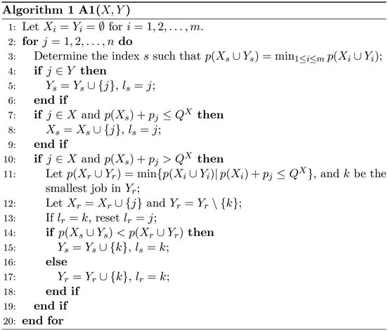
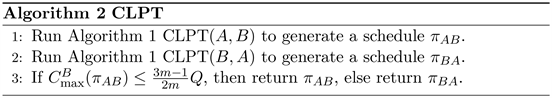
In Algorithm 1 there may be more than one machine each of which has the smallest load. A1 (X, Y) always chooses the one with the minimum index.

Algorithm 1 takes $O\left(m{n}^2\right)$ times. Therefore, the complexity of the CLPT algorithm is $O\left(m{n}^2\right)$ . In order to demonstrate the feasibility of the CLPT algorithm, we propose the following lemmas.

Lemma 1. In Algorithm 1, if $j\in X$ and $p\left(X_s\right)+p_j>Q^X$ , then $Y_i\ne \varnothing$ for any i with $p\left(X_i\right)+p_j\le Q^X$ .

Proof. Since $p\left(X_s\cup Y_s\right)={\min }_{1\le i\le m}p\left(X_i\cup Y_i\right)$ , we have

$p\left(X_i\cup Y_i\right)+p_j\ge p\left(X_s\cup Y_s\right)+p_j>Q^X.$

Then, $Y_i\ne \varnothing$ .¨

Lemma 2. For any $j\in X$ , Algorithm 1 can always find $X_r$ such that $p\left(X_r\right)+p_j\le Q^X$ .

Proof. Suppose to the contrary that $j\in X$ is the first job that cannot be assigned to any $X_i$ in Algorithm 1. Then, after jobs $\mathrm{1,2,}\cdots \mathrm{,}j-1$ are assigned, it holds that

$p\left(X_i\right)+p_j>Q^X,i=1,2,\cdots ,m.$ (4)

Denote $I=X\cap \left\{1,2,\cdots ,j-1\right\}={\displaystyle {\cup }_{i=1}^m{X}_i}$ . We have

$\begin{array}{c}p\left(I\right)+m{p}_j={\displaystyle \underset{i=1}{\overset{m}{\sum }}}p\left(X_i\right)+m{p}_j\\ >m{Q}^X\\ \ge \frac{3m}{2m+1}p\left(X\right)\\ \ge \frac{3m}{2m+1}p\left(I\right)+\frac{3m}{2m+1}{p}_j.\end{array}$

Equivalently, it holds that

$2p_j>\frac{p\left(I\right)}{m}=\frac{1}{m}{\displaystyle \underset{i=1}{\overset{m}{\sum }}}p\left(X_i\right),$

which implies that some X_is have at most one job of I, and no X_is have three or more jobs. Since $Q^X\ge {\max }_{i\in I}{p}_i$ , (4) implies that each X_i contains at least one job of I. Without loss of generality, we assume that $X_1\mathrm{,}{X}_2\mathrm{,}\cdots \mathrm{,}{X}_u$ each have one, and $X_{u+1}\mathrm{,}{X}_{u+2}\mathrm{,}\cdots \mathrm{,}{X}_m$ each have two jobs of I. Since job j is not longer than any job of I, the jobs in $X_1\mathrm{,}{X}_2\mathrm{,}\cdots \mathrm{,}{X}_u$ must be longer than those in $X_{u+1}\mathrm{,}{X}_{u+2}\mathrm{,}\cdots \mathrm{,}{X}_m$ . Otherwise, job j can be assigned to some X_i among $X_1\mathrm{,}{X}_2\mathrm{,}\cdots \mathrm{,}{X}_u$ .

Now consider the situation applying LPT to the job set X. We can schedule the job subset I such that $M_i$ processes the job of X_i for $i=1,2,\cdots ,u$ , and $M_{u+1}\mathrm{,}{M}_{u+2}\mathrm{,}\cdots \mathrm{,}{M}_m$ each process two jobs of $X_{u+1}\mathrm{,}{X}_{u+2}\mathrm{,}\cdots \mathrm{,}{X}_m$ . Then, job j cannot be finished by time $Q^X$ in LPT, a contradiction with $Q^X\ge C_{LPT}^X$ .¨

3. Numerical Simulation

3.1. Compare the Performance between the CLPT Algorithm and the Optimal Solution

To illustrate the effectiveness of the CLPT algorithm, we randomly generate a small number of problems to compare the performance between the CLPT algorithm and the optimal solution. We define the number of machines m, the total jobs of two agents n, the range of the maximum and minimum processing time of randomly generated jobs $\Delta$ and the value of constraint Q, which is an upper bound for the makespan for agent B and we use $\alpha$ to express, if $Q=\left(aLB\mathrm{,}bLB\right)$ , where

$LB=\max \left\{\frac{p\left(B\right)}{m}\mathrm{,}\max \left(p_j^B\right)\right\}$

then $\alpha =\left(a\mathrm{,}b\right)$ . Define $Pr=\frac{C_{\max }^A\left(\text{CLPT}\right)}{C_{\max }^A\left(\pi \right)}$ . The experimental parameters followed by the average $\overline{Pr}$ for 100 replications for the integer programming model and the CLPT algorithm. The results are as follows:

In Table 1: the number of machines is set at three levels: 3, 4 and 5, the total jobs of two agents is set at three levels: 5m, 10m and 15m, the constraint of α is set at three levels (1, 1.2), (1.2, 1.5) and (1.5, 1.8) and the variation range of the maximum and minimum value of the randomly generated jobs processing time is set at three levels: (1, 5), (1, 10) and (1, 20).

It can be seen from the experimental results that when m, n, Δ are fixed, the average value of Pr increases with the increase of α. When m, n, α are fixed, the average value of Pr decreases with the increase of Δ; when m, α, Δ are fixed, the average value of Pr decreases with the increase of n; when n, Δ, α are fixed, the average value of Pr increases with the increase of m. In a word, in each case, the average value of Pr is very close to 1, which suggests that the results obtained by the CLPT algorithm is very close to the optimal solution. The results demonstrate that the CLPT algorithm is an effective algorithm.

3.2. Compare the Performance between the CLPT Algorithm and the A-LS Algorithm

The effectiveness and efficiency of heuristic algorithms in finding minimum makespan schedules was empirically evaluated by solving a large number of

Table 1. Result for the average $\overline{Pr}$ .

problems. In this section, we mainly describe the experimental framework used and the computational results.

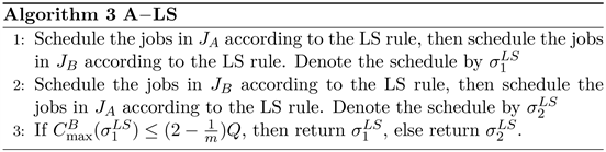
3.2.1. A-LS Algorithm

The LS (list-scheduling) rule is: whenever a machine becomes available, the algorithm iteratively assigns a list of jobs to the least loaded machine. Let we briefly review the A $-$ LS algorithm proposed by Zhao and Lu [1]

3.2.2. Experimental Framework

In order to compare the relative performance between the A-LS algorithm and the CLPT algorithm, we design three experimental frameworks. In each experiment, we investigate four variables: the number of machines m, the total jobs of two agents n, the value of constraint Q and the range of the maximum and minimum processing time of randomly generated jobs Δ. In order to investigate the effect of the investigated factors on the performance of the two algorithms, we use the control variable method to design experiments. For each fixed factors, we use Python 3.2 to generate at least 1000 instances randomly to observe the effect of the investigated factors on the results. The analysis of variance was appropriate in this case given equal samples and a large number of replications. Levene’s test was used to validate the assumption of homogeneous variance. Duncan’s post hoc test was used to rank the heuristics.

We define several parameters to compare the relative performance of the two algorithms. Let ${\rho }_1=\frac{C_{\max }^A\left(\text{CLPT}\right)}{C_{\max }^A\left(\text{LS}\right)}$ where ${\rho }_1\le 1$ means that the CLPT algorithm has a better performance than the A-LS algorithm, let ${\rho }_2=\frac{C_{\max }^B\left(\text{CLPT}\right)}{C_{\max }^B\left(\text{LS}\right)}$ where ${\rho }_2\le 1$ means that the CLPT algorithm violates fewer constraints than the A-LS algorithm. In order to show the relative performance between the two algorithms more intuitively. For each case, we generate 1000 instances randomly, among which:

· N1 represents the number of $C_{\max }^A\left(\text{CLPT}\right)<C_{\max }^A\left(\text{LS}\right)$ ;

· N2 represents the number of $C_{\max }^A\left(\text{CLPT}\right)>C_{\max }^A\left(\text{LS}\right)$ ;

· N3 represents the number of $C_{\max }^B\left(\text{CLPT}\right)<C_{\max }^B\left(\text{LS}\right)$ ;

· N4 represents the number of $C_{\max }^B\left(\text{CLPT}\right)>C_{\max }^B\left(\text{LS}\right)$ ;

· N5 represents the number of $C_{\max }^A\left(\text{CLPT}\right)\le C_{\max }^A\left(\text{LS}\right)$ and $C_{\max }^B\left(\text{CLPT}\right)\le C_{\max }^B\left(\text{LS}\right)$ ;

· N6 represent the number of $C_{\max }^A\left(\text{CLPT}\right)\ge C_{\max }^A\left(\text{LS}\right)$ and $C_{\max }^B\left(\text{CLPT}\right)\ge C_{\max }^B\left(\text{LS}\right)$ ;

The above six parameters can compare the performance of the CLPT algorithm and the A-LS algorithm intuitively. A higher value of N5-N6 indicates that the performance of the CLPT algorithm is better than that of the A-LS algorithm, and a higher value of N6-N5 indicates that the performance of the A-LS algorithm is better than that of the CLPT algorithm.

Table 2 presents a summary of all three experiments. In experiment E1, the number of machines m = 3, the total number of jobs is set at two levels???5m and 20m, the variation range of the maximum and minimum value of the randomly generated jobs processing time is set at four levels: (1, 2), (1, 5), (1, 10) and (1, 20), and the constraint of α is set at three levels: (1, 1.2), (1.2, 1.5) and (1.5, 1.8). In experiment E2, the number of machines is set at three levels: 3, 5 and 10, the total number of jobs is set at three levels: 5m, 10m and 20m, the Δ is set at two levels: (1, 5) and (1, 10), and the constraint of α is set at two levels: (1, 1.2) and (1.5, 1.8). In experiment E3, the number of machines is set at three levels: 3, 5 and 10, the number of jobs is fixed at n = 10m, the Δ is set at three levels: (1, 5), (1, 10) and (1, 20), and the constraint of α is set at two levels: (1, 1.2) and (1.5, 1.8). Under each parameter in all experiments, we generated 1000 instances randomly and calculated the number from N1 to N6 among these 1000 instances.

3.2.3. Computational Results

Table 3 gives the results of experiment E1. Table 3 shows the case of n = 5m and n = 20m. In case of m = 3, n = 5m: First, observe the effect of Δ on the results of the two algorithms. Table 3 shows that when Δ = (1, 2), α = (1, 1.8), N5-N6 Î [48, 118]; when Δ = (1, 5), α = (1, 1.8), N5-N6 Î [417, 429]; when Δ = (1, 10), α = (1, 1.8), N5-N6 Î [516, 530]. We can find that when m, n, α are fixed, the performance of the CLPT algorithm better than the A-LS algorithm increased as Δ increased.

Then, observe the effect of α on the results of the two algorithms. Table 3 shows that when Δ = (1, 2): α = (1, 1.2), N5-N6 = 118; α = (1.2, 1.5), N5-N6 = 48; α = (1.5, 1.8), N5-N6 = 91; when Δ = (1, 5): α = (1, 1.2), N5-N6 = 420; α = (1.2, 1.5), N5-N6 = 429; α = (1.5, 1.8), N5-N6 = 417; when Δ = (1, 10): α = (1, 1.2), N5-N6 = 530; α = (1.2, 1.5), N5-N6 = 530; α = (1.5, 1.8), N5-N6 = 516; when Δ = (1, 20): α = (1, 1.2), N5-N6 = 584; α = (1.2, 1.5), N5-N6 = 560; α = (1.5, 1.8), N5-N6 = 474. We can find that when m, n, Δ are fixed, the performance of the CLPT algorithm better than the A-LS algorithm decreased as α increased on the whole.

Table 2. Summary of the experimental frameworks.

Table 3. Result for experiment El.

In case of m = 3, n = 20m: First observe the influence of Δ on the results of the two algorithms. When Δ = (1, 2), α = (1, 1.8), N6-N5 Î [316, 367], which indicates that the A-LS algorithm outperformed the CLPT algorithm, and this advantage is very obvious. when Δ = (1, 5), α = (1, 1.8), N5-N6 Î [3, 12]; when Δ = (1, 10), α = (1, 1.8), N5-N6 Î [100, 161]; when Δ = (1, 20), α = (1, 1.8), N5-N6 Î [187, 218]. We can find that when m, n, α are fixed, the performance of the CLPT algorithm better than the A-LS algorithm increased as Δ increased, which is consistent with the results presented when m = 3, n = 5m. Then, we observe the effect of α. We can find that when m, n, Δ are fixed, the performance of the CLPT algorithm better than the A-LS algorithm decreased as α increased on the whole. which is also consistent with the results presented when m = 3, n = 5m.

Table 4 shows the results of experiment E2. Table 4 mainly observes the effect of the number of machines m and the number of jobs n on the experimental results. Since α and Δ have a great effect on the two algorithms, in order to avoid subjectivity, we set α at two levels: (1, 1.2) and (1.5, 1.8) and set Δ at two levels: (1, 5) and (1, 50).

In case of Δ = (1, 5), $\alpha =\left(\mathrm{1,1.2}\right)\cup \left(\mathrm{1.5,1.8}\right)$ : when m = 3, n = 5m, N5-N6 Î [380, 401]; when m = 3, n = 10m, N5-N6 Î [146, 220]; when m = 3, n = 20m, N5-N6 Î [−18, 32]. This indicates that when m, α, Δ are fixed, the performance of the CLPT algorithm better than the A-LS algorithm decreased as n increased. In particular, when m = 3, n = 20m, α = (1.5, 1.8), the performance of the A-LS algorithm is better than the CLPT algorithm. When m = 5, n = 5m, N5-N6 Î [477, 500]; when m = 5, n = 10m, N5-N6 Î [227, 284]; when m = 5, n = 20m, N5-N6 Î [66, 94]. This indicates that when m, α, Δ are fixed, the performance of the CLPT algorithm better than the A-LS algorithm decreased as n increased,

Table 4. Result for experiment E2.

which is consistent with the results presented when m = 3, n = 5m. When m = 10, n = 10m, the above results still holds. And we can also find that when n, Δ, α are fixed, the performance of the CLPT algorithm better than the A-LS algorithm increased as m increased on the whole.

In case of Δ = (1, 50), $\alpha =\left(\mathrm{1,1.2}\right)\cup \left(\mathrm{1.5,1.8}\right)$ : when m = 3, n = 5m, N5-N6 Î [497, 558]; when m = 3, n = 10m, N5-N6 Î [302, 380]; when m = 3, n = 20m, N5-N6 Î [160, 213]. This indicates that This indicates that when m, α, Δ are fixed, the performance of the CLPT algorithm better than the A-LS algorithm decreased as n increased, which is consistent with the results presented when Δ = (1, 5), $\alpha =\left(\mathrm{1,1.2}\right)\cup \left(\mathrm{1.5,1.8}\right)$ . When m = 5 and m = 10, the above results still holds. By comparing Δ = (1, 5) and Δ = (1, 50), it can be found that when Δ increases from (1, 5) to (1, 50), the value of N5-N6 also increases gradually, which is consistent with the results presented in Table 3. Moreover, when Δ = (1, 50), the number of machines m ≥ 5 and the number of jobs is greater than 20m, N6 is always equal to 0, which clearly indicates that the performance of the CLPT algorithm outperformed the A-LS algorithm in this case.

Table 5 shows the results of experiment E3. Table 5 mainly observes the effect

Table 5. Result for experiment E3.

of Δ on the experimental results. Because α has a significant effect on the experimental results, to avoid subjectivity, we set α = (1, 1.2) and α = (1.5, 1.8).

In case of α = (1, 1.2), n = 10m. When m = 3: Δ = (1, 5), N5-N6 = 217; Δ = (1, 10), N5-N6 = 253; Δ = (1, 20), N5-N6 = 380. When m = 5: Δ = (1, 5), N5-N6 = 270; Δ = (1, 10), N5-N6 = 337; Δ = (1, 20), N5-N6 = 373. When m = 10: Δ = (1, 5), N5-N6 = 306; Δ = (1, 10), N5-N6 = 300; Δ = (1, 20), N5-N6 = 275. We can find that when m, n, α are fixed, the range of N5-N6 increased as Δ increased on the whole and when n, Δ, α are fixed, the range of N5-N6 increased as m increased on the whole, which are consistent with the results presented in Table 3 and Table 4.

In case of α = (1.5, 1.8), n = 10m. When m = 3: Δ = (1, 5), N5-N6 = 167; Δ = (1, 10), N5-N6 = 287; Δ = (1, 20), N5-N6 = 302. When m = 5: Δ = (1, 5), N5-N6 = 194; Δ = (1, 10), N5-N6 = 288; Δ = (1, 20), N5-N6 = 262. When m = 10: Δ = (1, 5), N5-N6 = 242; Δ = (1, 10), N5-N6 = 251; Δ = (1, 20), N5-N6 = 246. We can find that the number of machines and Δ have the same effect on the experimental results of the two algorithms as the case of α = (1, 1.2), n = 10m. By comparing α = (1, 1.2) and α = (1.5, 1.8), we can study the effects of constraint α on the experimental results. It is found that the result of α = (1, 1.2) is better than that of α = (1.5, 1.8), which is also consistent with the results presented in Table 3 and Table 4.

3.2.4. Summary of Results

As expected, in most case, N1 ≥ N2, N3 ≥ N4, N5 ≥ N6, Which shows that the CLPT algorithm outperformed the A-LS algorithm. The data results show that among the four parameters: the number of machines m, the total job of two agents n, the constraint α and the Δ, the α and the Δ have significant effects on the results of the experiment. We can find that when m, n, α are fixed, the range of N5-N6 increased as the range of Δ increased on the whole and when n, Δ, α are fixed, the range of N5-N6 decreased as α increased on the whole.

4. Conclusions and Suggestions

This paper presents a new heuristic algorithm CLPT for the problem $P\mathrm{<mo>\; |\; </mo>\; <mo>\; |\; </mo>}{C}_{\max }^A\mathrm{<mo>\; :\; </mo>}{C}_{\max }^B\le Q$ . Firstly, in order to study the relative performance between the CLPT algorithm and the optimal solution, we design the integer programming model to obtain the optimal solutions in small scale cases. The experimental results show that the result obtained by the CLPT algorithm is very close to the optimal solution. Then, we design three experimental frameworks to compare the relative performance between the A-LS algorithm and the CLPT algorithm. The experimental results show that the CLPT algorithm outperformed the A-LS algorithm.

Several issues are worthy of future investigations. Firstly, it can be seen from the experimental results of the CLPT algorithm that the makespan of agent A

obtained by the CLPT algorithm is no more than $\frac{3m-1}{2m}$ times the optimal value, while the makespan for agent B is no more than $\frac{3m-1}{2m}$ times the threshold value. This provides a research direction: to prove that the performance ratio of the CLPT algorithm for this problem is $\left(\frac{3m-1}{2m}\mathrm{,}\frac{3m-1}{2m}\right)$ , which is a

better performance ratio than the one currently exists. Secondly, we can extend the two-agent scheduling problem to the model of multi-agent scheduling problem. Finally, we can also consider changing the objective function of each agent, such as changing the maximum completion time to the sum of completion time, the sum of weighted completion time and a linear combination of two agents.

Conflicts of Interest

The authors declare no conflicts of interest regarding the publication of this paper.

References

[1]	Zhao, K.J. and Lu, X.W. (2016) Two Approximation Algorithms for Two-Agent Scheduling on Parallel Machines to Minimize Makespan. Journal of Combinatorial Optimization, 31, 260-278. https://doi.org/10.1007/s10878-014-9744-y
[2]	Graham, R.L., Lawler, E.L., Lenstra, J.K. and Rinnooy Kan, A.H.G (1979) Optimization and Approximation in Deterministic Sequencing and Scheduling: A Survey. Annals of Discrete Mathematics, 5, 287-326. https://doi.org/10.1016/S0167-5060(08)70356-X
[3]	Baker, K.R. and Smith, J.C. (2003) A Multiple-Criterion Model for Machine Scheduling. Journal of Scheduling, 6, 7-16. https://doi.org/10.1023/A:1022231419049
[4]	Agnetis, A., Mirchandani, P.B., Pacciarelli, D. and Pacifici, A. (2004) Scheduling Problem with Two Competing Agents. Operations Research, 52, 229-242. https://doi.org/10.1287/opre.1030.0092
[5]	Agnetis, A., Pacciarelli, D. and Pacifici, A. (2007) Multi-Agent Single Machine Scheduling. Annals of Operational Research, 150, 3-15. https://doi.org/10.1007/s10479-006-0164-y
[6]	Balasubramanian, H., Fowler, J., Keha, A. and Pfund (2009) Scheduling Interfering Job Sets on Parallel Machines. European Journal of Operational Research, 199, 55-67. https://doi.org/10.1016/j.ejor.2008.10.038
[7]	Zhao, K.J. and Lu, X.W. (2013) Approximation Schemes for Two-Agent Scheduling on Parallel Machines. Theoretical Computer Science, 468, 114-121. https://doi.org/10.1016/j.tcs.2012.11.002
[8]	Zhao, K.J., Lu, X.W. and Gu, M.Z. (2016) A New Approximation Algorithm for Multi-Agent Scheduling to Minimize Makespan on Two Machines. Journal of Scheduling, 19, 21-31. https://doi.org/10.1007/s10951-015-0460-y
[9]	Zhao, K.J., Lu, X.W. and Gu, M.Z. (2018) An Algorithm for Multi-Agent Scheduling to Minimize the Makespan on m Parallel Machines. Journal of Scheduling, 21, 483-492. https://doi.org/10.1007/s10951-017-0546-9