New Probability Distributions in Astrophysics: I. The Truncated Generalized Gamma ()
1. Introduction
The generalized gamma distribution (GG) was introduced by [1] and carefully analyzed by [2]. The GG has three-parameters and the techniques to find them is a matter of research, see among others [3] [4] [5]. A significant role in astrophysics is played by the luminosity function (LF) for galaxies and we present some models, among others, the Schechter LF, see [6], a two-component Schechter—like LF, see [7], and the double Schechter LF with five parameters, see [8]. Another approach starts from a given statistical distribution for which the probability density function (PDF) is known. We know that for a given PDF,
,
(1)
where L is the luminosity. A data oriented LF,
, is obtained by adopting
which is the normalization to the number of galaxies in a volume of 1 Mpc3
(2)
which means
(3)
The above line of research allows exploring the LF for galaxies in the framework of well studied PDFs. Some examples are represented by the mass-luminosity relationship, see [9], some models connected with the generalized gamma (GG) distribution, see [10] [11], the truncated beta LF, see [12], the lognormal LF, see [13], the truncated lognormal LF, see [14], and the Lindley LF, see [15].
This paper brings up the GG and introduces the scale in Section 2. The new double truncation for the GG and the GG with scale is introduced in Section 3. The derivation of the truncated GG LF is done in Section 4. Section 5 contains the application of the GG LF to galaxies and quasars as well the fit of the averaged absolute magnitude for QSOs as function of the redshift.
2. The Generalized Gamma Distribution
Let X be a random variable defined in
; the GG (PDF),
, is
(4)
where
(5)
is the gamma function, with
,
and
. The above PDF can be obtained by setting the location parameter equal to zero in the four parameters GG as given by [16], pag. 113. The GG PDF scale as
and the gamma PDF as
: the introduction of the parameter c increases the flexibility of the GG.
The GG family includes several subfamilies, including the exponential PDF when
and
, the gamma PDF when
and the Weibull PDF when
.
The distribution function (DF),
, is
(6)
where
is the incomplete Gamma function, defined by
(7)
see [17]. The average value or mean,
, is
(8)
the variance,
, is
(9)
The mode, M, is
(10)
The rth moment about the origin is,
, is
(11)
The information entropy, H, is
(12)
where
is the digamma or Psi function defined as
(13)
where
, see [17].
The Scale
In some applications it may be useful to have a scale, b, and therefore the GG PDF,
, is
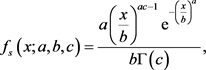 (14)
(14)
which has DF,  , as
, as
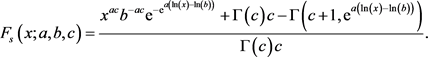 (15)
(15)
The average value,  , is
, is
 (16)
(16)
the variance,  , is
, is
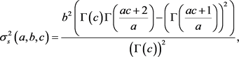 (17)
(17)
and the mode,  , is
, is
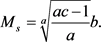 (18)
(18)
3. Double Truncation
Let X be a random variable defined in ; the new double truncated GG PDF,
  , can be found by evaluating of the following integral
 (19)
(19)
which is
 (20)
(20)
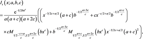
where  is the Whittaker M function, see Appendix A. We now define the constant of integration,
  , as
, as
 (21)
(21)
and as a consequence the truncated GG PDF is,  ,
,
 (22)
(22)
The average value, ![]() , is
, is
![]() (23)
(23)
where
![]() (24)
(24)
![]() (25)
(25)
![]() (26)
(26)
![]() (27)
(27)
The DF, ![]() , is
, is
![]() (28)
(28)
where
![]() (29)
(29)
![]() (30)
(30)
![]() (31)
(31)
The Scale
The truncated GG PDF with scale requires the evaluation of the following integral, ![]() ,
,
![]() (32)
(32)
which is
![]() (33)
(33)
The constant of integration, ![]() , is
, is
![]() (34)
(34)
and as a consequence the truncated GG PDF with scale is, ![]() ,
,
![]() (35)
(35)
The average value, ![]() is
is
![]() (36)
(36)
where
![]() (37)
(37)
![]() (38)
(38)
![]() (39)
(39)
![]() (40)
(40)
4. The Luminosity Function
In this section we present the Schechter LF, we derive the GG LF, we introduce the double truncation in the LF and we develop the adopted statistics.
4.1. The Schechter LF
The Schechter LF, introduced by [6], is
![]() (41)
(41)
here ![]() sets the slope for low values of L,
sets the slope for low values of L, ![]() is the characteristic luminosity and
is the characteristic luminosity and ![]() is the normalization. The luminosity density, j, is
is the normalization. The luminosity density, j, is
![]() (42)
(42)
The equivalent distribution in absolute magnitude is
![]() (43)
(43)
where ![]() is the characteristic magnitude as derived from the data. We now introduce the parameter h which is
is the characteristic magnitude as derived from the data. We now introduce the parameter h which is![]() , where
, where ![]() is the Hubble constant. The scaling with h is
is the Hubble constant. The scaling with h is ![]() and
and![]() .
.
4.2. Generalized Gamma LF
We replace in the GG with scale, see Equation (14) x with L (the luminosity), b with ![]() (the characteristic luminosity) and we insert
(the characteristic luminosity) and we insert ![]() which is the normalization to the number of galaxies in a volume of 1 Mpc3
which is the normalization to the number of galaxies in a volume of 1 Mpc3
![]() (44)
(44)
The magnitude version is
![]() (45)
(45)
where M is the absolute magnitude and ![]() is the characteristic magnitude. This four parameters LF, which was introduced in [10], was applied to the Sloan Digital Sky Survey (SDSS) in five different bands and to the near infrared band of the 2MASS Redshift Survey (2MRS), see [11].
is the characteristic magnitude. This four parameters LF, which was introduced in [10], was applied to the Sloan Digital Sky Survey (SDSS) in five different bands and to the near infrared band of the 2MASS Redshift Survey (2MRS), see [11].
4.3. Double Truncation for the LF
We replace in the truncated GG with scale, see Equation (35), x with L (the luminosity), b with ![]() (the characteristic luminosity),
(the characteristic luminosity), ![]() with
with ![]() (lower luminosity),
(lower luminosity), ![]() with
with ![]() (upper luminosity), and we insert the normalization,
(upper luminosity), and we insert the normalization, ![]() ,
,
![]() (46)
(46)
where ![]() is given by Equation (34). The luminosity density for the truncated GG LF,
is given by Equation (34). The luminosity density for the truncated GG LF, ![]() , has now a finite range of existence and is
, has now a finite range of existence and is
![]() (47)
(47)
The four luminosities ![]() and
and ![]() are connected with the absolute magnitudes M,
are connected with the absolute magnitudes M, ![]() ,
, ![]() and
and ![]() through the following relationship
through the following relationship
![]() (48)
(48)
where the indexes u and l are inverted in the transformation from luminosity to absolute magnitude and ![]() and
and ![]() are the luminosity and absolute magnitude of the sun in the considered band.
are the luminosity and absolute magnitude of the sun in the considered band.
The magnitude version of the truncated GG LF is
![]() (49)
(49)
![]() (50)
(50)
![]() (51)
(51)
The averaged absolute magnitude is
![]() (52)
(52)
4.4. The Adopted Statistics
The unknown parameters of the LF can be found through the Levenberg-Marquardt method (subroutine MRQMIN in [18] ) but the first derivative of the LF with respect to the unknown parameters should be provided. In the case of the truncated GG LF, see Equation (49), the first derivative with respect to the unknown parameters has a complicated expression, so we used the numerical first derivative. The merit function ![]() can be computed by
can be computed by
![]() (53)
(53)
where n is number of datapoints and the two indexes theo and astr stand for theoretical and astronomical, respectively. The residual sum of squares (RSS) is
![]() (54)
(54)
where ![]() is the theoretical value and
is the theoretical value and ![]() is the astronomical value. Particular attention should be paid to the number of unknown parameters in the LF: three for the Schechter function (formula (43)) and four for formula (49). The reduced merit function
is the astronomical value. Particular attention should be paid to the number of unknown parameters in the LF: three for the Schechter function (formula (43)) and four for formula (49). The reduced merit function ![]() can be computed by
can be computed by
![]() (55)
(55)
where![]() , n being the number of datapoints and k the number of parameters. The Akaike information criterion (AIC), see [19], is defined by
, n being the number of datapoints and k the number of parameters. The Akaike information criterion (AIC), see [19], is defined by
![]() (56)
(56)
where L is the likelihood function and k the number of free parameters in the model. We assume a Gaussian distribution for the errors and the likelihood
function can be derived by the ![]() statistic
statistic ![]() where
where ![]() has been computed by Equation (53), see [20] [21]. Now AIC becomes
has been computed by Equation (53), see [20] [21]. Now AIC becomes
![]() (57)
(57)
The Bayesian information criterion (BIC), see [22], is
![]() (58)
(58)
where L is the likelihood function, k the number of free parameters in the model and n the number of observations. The phrase “better fit” used in the following means that the three statistical indicators:![]() , AIC and BIC are smaller for the considered LF than for the Schechter function.
, AIC and BIC are smaller for the considered LF than for the Schechter function.
5. Astrophysical Applications
In this section we apply the truncated GG LF to the SDSS galaxies and to QSOs. The introduction of the redshift dependence for lower and upper absolute magnitude allows to model the average absolute magnitude versus redshift for QSOs.
5.1. SDSS Galaxies
In order to perform a test we selected the data of the Sloan Digital Sky Survey (SDSS) which has five bands ![]() (
(![]() ),
),![]() (
(![]() ),
),![]() (
(![]() ),
),![]() (
(![]() ) and
) and ![]() (
(![]() ) with
) with ![]() denoting the wavelength of the CCD camera, see [23]. The data of the astronomical LF are reported in [24] and are available at https://cosmo.nyu.edu/blanton/lf.html. The numerical values of the four parameters a, c,
denoting the wavelength of the CCD camera, see [23]. The data of the astronomical LF are reported in [24] and are available at https://cosmo.nyu.edu/blanton/lf.html. The numerical values of the four parameters a, c, ![]() and
and ![]() are given in Table 1.
are given in Table 1.
![]()
Table 1. Parameters for fits to LF in SDSS Galaxies with the four parameters truncated GG LF as represented by formula (49).
The Schechter function, the new four parameters function as represented by formula (49) and the data are reported in Figures 1-5, where bands![]() ,
, ![]() ,
, ![]() ,
, ![]() and
and ![]() are considered.
are considered.
Table 2 presents the luminosity density evaluated with the Schechter LF, j, and with the truncated GG LF, jT. The range of existence in the truncated case is finite rather than infinite and therefore the luminosity density is always smaller than in the standard case.
5.2. Luminosity Function for QSOs
For our first example, we selected the catalog of the 2dF QSO Redshift Survey (2QZ), which contains 22431 redshifts of QSOs with![]() , see [25]. We processed them as explained in [26]. A typical example of the observed LF for QSOs when
, see [25]. We processed them as explained in [26]. A typical example of the observed LF for QSOs when ![]() as well the fit with the four parameters truncated GG LF is presented in Figure 6 with data as in Table 3.
as well the fit with the four parameters truncated GG LF is presented in Figure 6 with data as in Table 3.
In the second example we explored the faint LF for quasars in the range of redshifts ![]() as given in Figure 4 of [27]. The results are displayed in Figure 7 with data as in Table 4.
as given in Figure 4 of [27]. The results are displayed in Figure 7 with data as in Table 4.
5.3. Average Absolute Magnitude versus Redshift
The first application is about galaxies: we processed the SDSS Photometric Catalogue DR 12, see [28], which contains 10,450,256 galaxies (elliptical + spiral) with redshift and rest frame ![]() absolute magnitude. The lower absolute magnitude is fixed at
absolute magnitude. The lower absolute magnitude is fixed at ![]() and the upper absolute magnitude is the maximum absolute magnitude of the selected bin in redshift. The above choice adopts the SDSS DR12 cosmological evaluation of the absolute magnitude. Figure 8 displays averaged absolute magnitude, theoretical averaged absolute magnitude, lower and upper limit in absolute magnitude functions of the redshift.
and the upper absolute magnitude is the maximum absolute magnitude of the selected bin in redshift. The above choice adopts the SDSS DR12 cosmological evaluation of the absolute magnitude. Figure 8 displays averaged absolute magnitude, theoretical averaged absolute magnitude, lower and upper limit in absolute magnitude functions of the redshift.
![]()
Figure 1. The luminosity function data of SDSS(u*) are represented with error bars. The continuous line fit represents the four parameters truncated GG LF (49) and the dotted line represents the Schechter function.
![]()
Figure 2. The luminosity function data of SDSS(g*) are represented with error bars. The continuous line fit represents the four parameters truncated GG LF (49) and the dotted line represents the Schechter function.
![]()
Table 2. Luminosity density in SDSS Galaxies evaluated with the Schechter LF, formula (42), and with the four parameters truncated GG LF, formula (47), when ![]() and
and![]() .
.
![]()
Figure 3. The luminosity function data of SDSS(r*) are represented with error bars. The continuous line fit represents the four parameters truncated GG LF (49) and the dotted line represents the Schechter function.
![]()
Figure 4. The luminosity function data of SDSS(i*) are represented with error bars. The continuous line fit represents the four parameters truncated GG LF (49) and the dotted line represents the Schechter function.
![]()
![]()
Table 3. The four parameters truncated GG LF as represented by formula (49) in the QSO case.
![]()
Table 4. The four parameters truncated GG LF as represented by formula (49) for QSOs in the COSMOS field.
![]()
Figure 5. The luminosity function data of SDSS(z*) are represented with error bars. The continuous line fit represents the four parameters truncated GG LF (49) and the dotted line represents the Schechter function.
![]()
Figure 6. The observed LF for QSOs, empty stars with error bar, when z [0.3, 0.5] and M [−24.93, −22.29]. The continuous line fit represents the four parameters truncated GG LF (49).
![]()
Figure 7. The observed LF for QSOs in the COSMOS field, empty stars with error bar, when z [3.7, 4.7] and M [−28, −22]. The continuous line fit represents the four parameters truncated GG LF (49).
The second application is about the QSO and we used the framework of the flat cosmology in order to find the absolute magnitude relative to the catalog of the 2dF QSO Redshift Survey (2QZ), exactly as [26]. The two cosmological parameters are ![]() and
and![]() , where
, where ![]() is the Hubble constant expressed in kms−1Mpc−1, and
is the Hubble constant expressed in kms−1Mpc−1, and ![]() is
is
![]() (59)
(59)
where G is the Newtonian gravitational constant and ![]() is the mass density at the present time. A useful reference for the upper magnitude as function of the redshift can be obtained from the distance modulus as given by Equation (5) in [26] once the limiting magnitude of the sample 2QZ,
is the mass density at the present time. A useful reference for the upper magnitude as function of the redshift can be obtained from the distance modulus as given by Equation (5) in [26] once the limiting magnitude of the sample 2QZ, ![]() , is adopted
, is adopted
![]() (60)
(60)
The above equation represents a useful theoretical reference. Another, more empirical, way explores numerically the maximum and the minimum in absolute magnitude functions of the redshift for the sample 2QZ. In order to fix the numbers we fitted the upper absolute magnitude with the third degree polynomial
![]() (61)
(61)
with![]() ,
, ![]() ,
, ![]() and
and![]() . The lower absolute magnitude is fitted with the second degree polynomial
. The lower absolute magnitude is fitted with the second degree polynomial
![]() (62)
(62)
with![]() ,
, ![]() and
and![]() . Another useful relation is
. Another useful relation is
![]()
Figure 9. Average observed absolute magnitude versus redshift for QSOs (red points), average theoretical absolute magnitude for the four parameters of the truncated GG LF as given by Equation (52) (dot-dash-dot green line), the lowest absolute magnitude at a given redshift as given by the sample (full black line) and the highest absolute magnitude at a given redshift as given by the sample (dashed black line); RSS = 1.62.
![]() (63)
(63)
Now different combinations of curves can be used. Figure 9 presents the combination which minimizes the RSS.
6. Conclusions
Truncated GG: We derived an expression for the left and right truncated GG PDF in terms of the Whittaker M function, see Equation (22), its DF, see Equation (28), and its average value, see Equation (23).
Truncated LF: The truncated LF for galaxies or QSO is derived both in the luminosity form, see Equation (46), and in the magnitude form, see Equation (49). In all the astrophysical examples here analyzed which are the five bands of SDSS galaxies, see Table 1, the QSOs when![]() , see Table 3, and the faint LF for QSOs in the range of redshift
, see Table 3, and the faint LF for QSOs in the range of redshift![]() , see Table 4, the
, see Table 4, the ![]() of the truncated GG is smaller than the Schechter LF. Table 2 presents the luminosity density in SDSS Galaxies with a finite range of existence rather than infinite.
of the truncated GG is smaller than the Schechter LF. Table 2 presents the luminosity density in SDSS Galaxies with a finite range of existence rather than infinite.
Average Magnitude versus redshift: The averaged absolute magnitude of the SDSS galaxies and QSOs belonging to the catalog 2QZ as functions of the redshift are reasonably fitted by the averaged absolute magnitude of the truncated GG LF, see Equation (52). In order to perform the fit we provided for ![]() a redshift dependence, see Equation (63), and we inserted as lower and upper absolute magnitudes those given by the minimum and maximum values of the selected bin in redshift.
a redshift dependence, see Equation (63), and we inserted as lower and upper absolute magnitudes those given by the minimum and maximum values of the selected bin in redshift.
Appendix A: The Whittaker M function
The Whittaker M function, ![]() , solves the differential equation
, solves the differential equation
![]() (A1)
(A1)
The regularized hypergeometric function, ![]() , as defined by the Gauss series, is
, as defined by the Gauss series, is
![]() (A2)
(A2)
where![]() , and
, and ![]() is the Pochhammer symbol
is the Pochhammer symbol
![]() (A3)
(A3)
The generalized hypergeometric series is denoted by ![]() and the case
and the case ![]() and
and ![]() gives
gives
![]() (A4)
(A4)
The relationship
![]() (A5)
(A5)
allows to express the Whittaker M function in terms of the generalized hypergeometric function, ![]() , see [17] [29].
, see [17] [29].