A Note on Densities of the L2 Mental Lexicon Network

Yusuke Higuchi¹, Rumi Takahashi², Mikihiro Tanaka³

¹Mathematics Laboratories, College of Arts and Sciences, Showa University, Yamanashi, Japan.
²Fuculty of Arts and Sciences, Showa University, Yamanashi, Japan.
³Department of English Language and Culture, Konan Women’s University, Hyogo, Japan.

DOI: 10.4236/ojml.2019.96037                

Abstract

In this note, we discuss a supplementary explanation about works of Takahashi and Tanaka, which are a kind of replication study of Wilks & Meara (2002), where they discuss the structure of learners’ mental lexicon network from the viewpoint of psycholinguistics. Here we mainly discuss some mathematical structures which support their studies latently. Using some simple random graph techniques, we propose that the role of “densities” is important and useful under some suitable assumptions. Then, we exhibit the effectiveness of our method by applying it to the data of experiments in Takahashi and Tanaka, where some inequalities obtained mathematically help us to investigate some of the aspects of the L2 mental lexicon network. Mathematical proofs and detailed discussion are collected in the final section, in which we give also mathematical interpretation on some models which were shown by computer simulations in previous works.

Keywords

Mental Lexicon, Random Graph, Density, Complex Network, Second Language, Mathematical Modelling

1. Introduction

The basic object to examine “mental lexicon” is to investigate how humans organize huge “words” in their mind. Many researchers in various areas are attracted to the structure of mental lexicon and try to illustrate it. Many types of findings are found in the standard textbooks, for example, (Aitchison, 1987, 2012) and (Boyd, 1993); an overview of various fields on psycholinguistics including mental lexicon is found in (Gaskell, 2009). There exist various methods or ideas due to the difference of the communities where researchers belong to, but no one will imagine each word in the mental lexicon is completely isolated. Thus it is natural to consider words are linked one another and the whole words form “word-web”, a kind of network. In this sense, a model of the mental lexicon becomes a network, that is, graph; a graph is a notion in mathematics and constructed by vertices corresponding to “words” and edges corresponding to relationships among words. Classically graphs are known to be applied effectively to chemistry, physics, social science and so on. Also in the context of linguistics and psychology, there exist many works on graph-theoretical mental lexicon. For instance, refer to (Kiss, 1968; Meara, 1992; Rapaport, Livant, & Boyd, 1966; Scott, 1991; Wilks & Meara, 2002; Wilks & Meara, 2007; Wilks, Meara, & Wolter, 2005). In many works, graph-invariants, which are some stable quantities measuring a given graph, in the structure of mental lexicon are discussed: the distribution of degrees, cluster coefficient, path length, community and so on. See also Marcus (2001) for the study on the mental lexicon with computer sciences. Moreover, after the original idea of complex network, or, scale-free network are brought by Barabási & Albert (1999) and Barabási (2009), one can see this concept describes many phenomena in sociology, biology or economics well. Therefore many researchers try to apply it to the mental lexicon: (Gruenenfelder & Mueller, 2007; Gruenenfelder & Pisoni, 2005, 2009; Schur, 2007; Stella, Beckage, Brede, & De Domenico, 2018; Vitevitch, 2008; Vitevitch, Goldstein, Siew, & Castro, 2014), for instance. In summary, graph-theoretical approach for the mental lexicon has been well developed.

However, there is considerable disagreement over how the mental lexicon is constructed in human mind. In particular, it is not clear how different the mental lexicons between first language (L1) and second language (L2) are. Refer to, for instance, (Harley, 2010) for the mental lexicon for bi- or multi-lingual. Theoretically it is discussed that the link occurs between two words when they have some semantic relationship, and that co-ordination or collocation is stronger than others, superordination or synonymy, for instance, (Aitchison, 1987, 2012); this seems to be agreed for L1. However, no one may know whether this holds or not for L2; the co-ordination or collocation may be stronger in the semantic relation, or, the syntactical or phonological relation may be stronger than the semantic one, or, the relation in the wide meaning of “co-occurrence” may be stronger than others. Then, to examine how humans link among words actually and the mental lexicon for L1 and/or L2, we believe we should pursue phycholinguistic experiments. In the word association task of Wilks and Meara (Wilks & Meara, 2002), participants were 30 learners of French whose L1 was English and 30 native speakers of French and were asked to identify associations from a given set of randomly chosen five French words. These experiments bring the number of “hits”, that is, pairs of associated words, for each participant, then we know, as a result, native speakers than nonnative ones perceive significantly more associations. This simple experiment gives to us slight information on how the L2 mental lexicon is organized; that is, “densities” in word associations are different between L1 and L2 since the network of word associations is considered to be denser as the number of word associations increases. Thus main conclusion in (Wilks & Meara, 2002) is that L1 networks are denser than L2 networks of the learners in French. We should remark the linkage “association” in (Wilks & Meara, 2002) depends on the individual impression of each participant, that is, we cannot know what type of reasons generates their links. In other words, it is natural to investigate the L2 mental lexicon without any restriction in a way to associate.

Following the work stated above, Takahashi and Tanaka (Takahashi & Tanaka, in preparation; Tanaka & Takahashi, 2019) try to investigate how the L2 lexical network is organized in English, where some mathematical methods essentially help them to state conclusions but explicit expressions and details are hidden since their discussion should have been done mainly in the context of (psycho)linguistics. Therefore one of the main objects of this paper is to give a supplementary explanation on mathematical ideas used in (Takahashi & Tanaka, in preparation; Tanaka & Takahashi, 2019) explicitly. To investigate the structure of the mental lexicon as a network, we need many psychological experiments for a large number of persons and many tools guaranteed theoretically for analysing properties of the model. As a first step, our methods with mathematically rigorous discussion in the sense of random graph, which are quite basic and useful, will be more developed in the future research.

This paper is organized as follows: In Section 2, we briefly review the study of Wilks & Meara (2002) (Section 2.1) and explain their methods in terms of graph theory and random graphs (Subsection 2.2). We discuss the main study in this paper in Section 3: firstly the brief review of the studies of Takanashi and Tanaka (Takahashi & Tanaka, in preparation; Tanaka & Takahashi, 2019) is given in Subsection 3.1. Then we explain some latent mathematical ideas for (Takahashi & Tanaka, in preparation; Tanaka & Takahashi, 2019) in Subsections 3.3. After that, we propose and apply our methods to the data of experiments in (Takahashi & Tanaka, in preparation; Tanaka & Takahashi, 2019) in Subsection 3.4. Finally we discuss concluding remarks about our methods and mental lexicon networks of L2 learners’ in Section 4. Some supplements in the text (some mathematical proofs, some sample of experiments in (Takahashi & Tanaka, in preparation; Tanaka & Takahashi, 2019), mathematical interpretations and so on) are exhibited in the Appendix.

2. Background

2.1. The Study of Wilks and Meara

In this paper, our methods are almost the same as in (Wilks & Meara, 2002). In a given set of words, one construct a kind of network of words individually; such a network is so-called a graph. Here the set of vertices (in the terms of Graph Theory) corresponds to that of words and the set of edges does to that of “associations”, where association implies the existence of strongly link of two words. The density of a given graph is defined as the ratio of the number of all the edges in the number of all possible edges which equals to $n\left(n-1\right)/2$ , where n is the number of all the words. Wilks & Meara (2002) investigated a difference between the densities of L1 and L2 in French. Their experiment was designed as 40 questions (items) in one questionnaire and each question is: for 5 words chosen randomly from the first 1000 most frequency words,

1) if any pair of 5 words are thought to be no association, nothing should be written;

2) if one or more pairs of 5 words are thought to be associated, the only one pair of strongest association should be circled.

We say the “hit rate” for the ratio of the number of answers to be associated over that of all questions.

Through this “five-word task” experiment, we should remark that we cannot obtain the structure of associations of the individual mental lexicon network since, under the instruction (2), we can only see the strongest link pair of two words; so to say, we asked the participant to break the “detail structure” of associations. However, it is important to see the ratio of items with no-association. Once the network of mental lexicon was constructed, the density p behaves like the existence probability of association between any pair of words in this network. Under the assumption that such a probability p is identically and independent distributed, the probability of an item with no-association occurring is estimated as ${\left(1-p\right)}^{10}$ since the number of all possible pairs is 10. Therefore, by observing the ratio of items with no-association, we can get the density p. We are very careful to treat items with association, which was forced to be indicated one-pair only.

Of course, we know such instruction (2) may be suitable for actual experiment with psychological reasons for participants. If such a experiment was done for subjects not having human emotions, for example, in computer simulations, the restriction in (2) would not be needed. Namely, instead of (2), if the condition that all pairs of association might be indicated was asked, it would be somewhat difficult for participants to choose “no-association” in the item just after indicating “many associations”.

Repeatedly we should say it is important to obtain the number of items with no-association as accurately as possible.

2.2. Random Graphs

2.2.1. Interpretation of the Setting of Wilks and Meara

Among huge words in one’s mind, it is natural to consider a kind of network of words, mental lexicon network, is constructed, and some associations appear and other ones disappear every time one sees or hears words. Namely, such a network will be drastically changing its structure depending on the input of words. However, once the context generating words is confirmed, it is considered to be almost stable with small fluctuation. On the other hand, how does the network of “mental lexicon” behave every time words are given randomly without any context? We believe the network appearing in such a situation may be a “basic” or “core in (Wilks & Meara, 2002)” mental lexicon; although it will change its structure at every input of words, its density is considered to be stable in the same way as in (Wilks & Meara, 2002), where they actually examined to compare the relative densities of first language (L1) in French and second language (L2) in such “basic” lexical networks. Here the word “density” can be treated as the proportion of the number of the associated word pairs over the number of all possible pairs in the whole given words. In addition, its “density” can correspond to a probability p; if a pair of words is chosen randomly, they will associate each other with probability p. The model of network with probability is usually said to be a random graph in mathematics. In particular, the Erdös-Rényi model is well-known and much research on it have been actively studied; the first remarkable paper about this model is appeared in (Erdös & Rényi, 1959). Once the density, or probability, is given, we can generate a sample network of mental lexicon in the context of random graphs. The set of words and that of associations are the set of vertices and edges in the term of graph theory, respectively. Then $G\left(n,p\right)$ denotes a random “undirected” graph such that every possible edge occurs independently with probability $0<p<1$ for n vertices. See also Figure 1.

In Wilks and Meara (Wilks & Meara, 2002), they derived the density by many computer simulations to generate regular random graphs and observe the existence of edges in randomly selected subgraph of 5 vertices. However, we emphasize the relationship between a hit rate and its density can be obtained analytically, whose concrete form will be seen in Proposition 2.1 in Section 2.2.2. Namely, once we obtained the hit rate, we can derive its density immediately. In this sense, we calculated the densities in the paper of Wilks and Meara, then their evaluations were about half of our ones. We imagine there was a little bit of mistake or ambiguity in generating random “regular” graphs in their paper. They introduced all notions in graph theory in terms of “undirected” graph: for instance, symmetric adjacency matrices representing the structure of undirected graphs, the density represented by the ratio of the number of all undirected edges in the complete graph and so on. So it is natural to recognize their results in the setting “undirected” graphs. In fact, we re-examined their strategy in using a statistical programming language R (R Core Team, 2019) and a graph theoretical package iGraph (Csardi & Nepusz, 2006), then our estimation seems to be right. However the essence and importance of their paper cannot suffer from tiny errors;

Figure 1. Samples of random graphs of 20 vertices, G(20, p): Edge probabilities p are set as 0.7. 0.5, 0.15, 0.08 and 0.03, respectively.

as will be seen in Remark 2.4, if we apply “directed” random graphs to the association task for 5 words chosen randomly in (Wilks & Meara, 2002), we can find the estimations in our way coincide with the results in their simulation.

2.2.2. Basic Relations around Densities

As stated in the above, we first give a simple relation between the hit rate in the five-word task and the density.

Proposition 2.1. We can easily find, for the five-word task,

$“\text{hitrate}”=1-{\left(1-“\text{density}”\right)}^{10}.$ (1)

Thus, once the hit rate is given from actual experiments, we soon obtain the density as

$“\text{density}”=1-{\left(1-“\text{hitrate}”\right)}^{\frac{1}{10}}.$ (2)

Here the exponent “10” of the right hand side of (1) comes from $\left(\begin{array}{l}5\hfill \\ 2\hfill \end{array}\right)$ in “five-word task,” which is the number of all possible pairs on one question consisting of 5 words chosen randomly. Thus, if we use a questionnaire such that each question consists of “ $n$ -words” ( $n\in N$ ) chosen randomly, that is, “ $n$ -word task,” each exponent of the right hand sides of (1) and (2) is replaced with $\left(\begin{array}{l}n\hfill \\ 2\hfill \end{array}\right)$ and $1/\left(\begin{array}{l}n\hfill \\ 2\hfill \end{array}\right)$ , respectively.

Before stating the next relation, we give a definition in terms of graph theory. The set of all words correspond to the set of vertices $V\left(G\right)$ of a given graph G. Similarly the set of all associations among words corresponds to the set of edges $E\left(G\right)$ and the density does to the ratio of the number of edges of G in that of the complete graph with size of $V\left(G\right)$ .

Definition 2.2 Let $G=\left(V\left(G\right),E\left(G\right)\right)$ be a finite simple undirected graph and let A be a non-empty proper subset of $V\left(G\right)$ and $B=V\left(G\right)\backslash A$ . Then we define four types of densities $p_{A+B},p_{AA},p_{BB}$ and $p_{AB}$ as follows:

$p_{A+B}=\frac{\#E\left(G\right)}{\left(\begin{array}{c}{n}_A+n_B\\ 2\end{array}\right)},p_{AA}=\frac{\#E\left(\langle A\rangle \right)}{\left(\begin{array}{c}{n}_A\\ 2\end{array}\right)},p_{BB}=\frac{\#E\left(\langle B\rangle \right)}{\left(\begin{array}{c}{n}_B\\ 2\end{array}\right)}\text{and}{p}_{AB}=\frac{\#E\left(A,B\right)}{n_A{n}_B},$ (3)

where $n_U$ is the number of elements of the set U, $\langle U\rangle$ is the subgraph of G induced by the set of vertices U and $E\left(A,B\right)$ is the set of edges connecting two set of vertices A and B.

We find the following relation is trivial from Definition 2.2 but important in this paper. It may be said to be a kind of mean field theoretic approximation; the left hand side of the following equation implies a “one-body system” A + B and the right hand a “two-body system” A and B.

Proposition 2.3 We have the relation among four densities as

$\left(\begin{array}{c}{n}_A+n_B\\ 2\end{array}\right)\cdot p_{A+B}=\left(\begin{array}{c}{n}_A\\ 2\end{array}\right)\cdot p_{AA}+n_A\cdot n_B\cdot p_{AB}+\left(\begin{array}{c}{n}_B\\ 2\end{array}\right)\cdot p_{BB}.$ (4)

Let us express the symbols shown in the above in the context of the word association, which will be discussed in Section 3: $n_A$ and $n_B$ are the numbers of words in Group A and Group B, respectively; thus $n_A+n_B$ indicates the numbers of the whole set of all words, Group A + B. Moreover, $p_{AA}$ , $p_{BB}$ , $p_{AB}$ and $p_{A+B}$ imply the densities connecting two words in Group A, in Group B, one word in Group A and the other in Group B, and in Group A + B, respectively. In actual experiments, we may say (4) becomes a kind of assumption for derived/underived “small” densities satisfying in the sense of mean field theoretic approximation. In particular, we discuss in Section 3 the relationship among densities in our “five-word task” experiments under the relation (4) for simplicity. For more details about the relation (4) in the “k-word task” experiments, refer to Section A3 in Appendix.

Remark 2.4. Throughout this paper, we treat “undirected” random graphs only. As stated in the previous subsection, “undirected” random graphs seemed to be treated in (Wilks & Meara, 2002). However, by seeing the differences between our estimations and their results and referring to the sequential works of Meara et al. (Wilks, Meara, & Wolter, 2005; Meara, 2007), we confirm they treated “directed” graphs, or, “digraphs” in their simulations. Now let us show the relationship between a hit rate and a density in the case of “digraphs” in the similar way to that in the above. Let $G=\left(V\left(G\right),A\left(G\right)\right)$ be a di-graph, where $A\left(G\right)$ is the set of all directed edges, or, arcs: $\left[x,y\right]\in A\left(G\right)$ implies $\left[x,y\right]$ is an arc from x to y. In this setting, it is natural that x and y in $V\left(G\right)$ are considered to be “associated” if and only if $\left[x,y\right]\in A\left(G\right)$ or $\left[y,x\right]\in A\left(G\right)$ . We set the density of a digraph $G=\left(V\left(G\right),A\left(G\right)\right)$ as

$p=\frac{\#A\left(G\right)}{\#V\left(G\right)\left(\#V\left(G\right)-1\right)}.$ (5)

Under the assumption that such a probability p is identically and independently distributed, the probability of no-association occurring between x and y is estimated as ${\left(1-p\right)}^2$ . Moreover we can easily find, for a randomly selected n-words experiment, that is, “n-word task,”

$“\text{hitrate}”=1-{\left(1-p\right)}^{2\left(\begin{array}{l}n\hfill \\ 2\hfill \end{array}\right)}.$ (6)

Thus, once the hit rate is given from actual experiments, we soon obtain the density p as

$p=1-{\left(1-“\text{hitrate}”\right)}^{\frac{1}{n\left(n-1\right)}}.$ (7)

When $n=5$ , we can see the formula (6) almost recovers the results of simulations in Table 1 and Figure 3 in (Wilks & Meara, 2002). In their sequential works (Wilks, Meara, & Wolter, 2005; Meara, 2007), they treat digraphs without ambiguity and introduce a modified model considering associations linked “indirectly” in some way. We give mathematical interpretations on some of their models and results in simulations in Section A6 in Appendix. Repeatedly we remark we treat “undirected” random graphs only in this paper.

3. Main Study

3.1. The Study of Takahashi and Tanaka

The studies in (Takahashi & Tanaka, in preparation; Tanaka & Takahashi, 2019) report on a word association task for Japanese learners who learn English as an L2. The English words used in our word association task were chosen from The New JACET List of 8000 Basic Words (JACET, 2016), which is a list of essential English vocabulary for university students in Japan. In total, we chose 1090 words essential for junior high school students and 1744 words essential for senior high school students; hereinafter the former set of words is called “Group A”, the latter “Group B”, and the whole set of words “Group A + B.” The format of our word association task was similar to the one performed in Wilks and Meara (Wilks & Meara, 2002). However, we performed it using English words instead of French words. In the experiment, we presented a set of five words in each trial. See also Figure 2. There were 80 word sets in a word association test as follows: in the word set 1 - 40, we selected 5 words randomly from Group A + B; in the word set 41 - 80, we chose 5 words only from Group B; the two types of words sets appeared in a random order in each questionnaire. Participants were asked to identify a single association, if any, in a given set of randomly chosen five words in the word association tests that we devised. Then we measured the “hit rate”, the ratio of word associations. An example and the flow of our actual experiment can be found in Section A1.

In (Takahashi & Tanaka, in preparation), the participants were five Japanese undergraduate students whose proficiency level of English was intermediate (their TOEIC Listening and Reading score was approximately 600), and five Japanese researchers who used English on daily basis in their research. The data of the students showed that the mean hit rate was higher when the words from Group A were included, suggesting that the words in Group A might be functioning as hub vertices that help link the words in the lexical network in their L2 mental lexicon. See also Figure 3. This tendency was not observed in the test results of the researchers. See also Table 1.

In Tanaka & Takahashi (2019), the participants were thirty-two native

Table 1. Result in (Takahashi & Tanaka, in preparation).

Figure 2. An example of associations in given five words.

Figure 3. Sample of another kind of random graph: Group A (white-squared 10 vertices) and Group B (black-circled 20 vertices); Edge probabilities in two vertices within A, within B, and between A and B, are set as 0.15, 0.08, and 0.11, respectively.

Table 2. Result in (Tanaka & Takahashi, 2019).

speakers of Japanese whose proficiency level of English was also intermediate and their TOEIC Listening and Reading score was approximately 400 in average. We found a significant difference between the mean hit rate in Group A + B (68%) and that in Group B (60%, p < 0.001). This suggests that the ratios of how one word is associated with another are different in Group A and Group B. See also Table 2. In addition, we found that estimated densities for word associations were 0.11 for Group A + B, whereas 0.09 for Group B, which might indicate that the word associations involving Group A were denser than those in Group B.

For interpretation and analysis in terms of (psycho)linguistics for these results, refer to (Takahashi & Tanaka, in preparation; Tanaka & Takahashi, 2019). We should remark that the young participants selected for our experiments in (Takahashi & Tanaka, in preparation; Tanaka & Takahashi, 2019) are intermediate-level learners of English in a Japanese university. We believe participants must not be too high-grade nor low-grade in investigating the standard structure of the L2 mental lexicon for the majority. In this sense, our participants might be quite suitable.

3.2. Taste of Scale-Free Network

The concept of complex networks, or, scale-free network has relied on the construction of network evolution models. Most of studies on complex network, which are based on (Barabási, 2009; Barabási & Albert, 1999), discuss the topological statistics of the evolving network.

In our studies, we cannot evaluate such properties since the number of vertices, or equivalently, words, is very large but fixed. However we imagine the mental lexicon network of L2 learner may evolve like a complex network evolution model as they acquire new words more and more. In this sense, we can say that we could see some snapshot in their evolution and some trend as complex network. Thus, through the actual experiment, we would find the existence of “hubs”, which correspond to “important words” in the process of acquiring words.

Let us assume that Group A is the set of “more important” words in the whole set of words Group A + B. If this assumption is true, we can find the significant differences between the hit rates of Group A + B and Group B; moreover the density involving Group A is denser than that involving Group B. In other words, the significant differences can be said to be in favour of complex network in the process of L2 learners’ mental lexicon evolution model. However, we cannot state that the mental lexicon forms the scale-free network due to lack of showing the scale-free properties (Barabási, 2009; Barabási & Albert, 1999; Schur, 2007; Vitevitch, Goldstein, Siew, & Castro, 2014), for example, a power law distribution of degree of vertices. At this stage, all we can say is that the L2 mental lexicon network has a possibility to be a kind of scale-free network. Here let us recall our main purpose is to show that the whole set of words can be divided into more and less important groups and to propose some modelling for our experiment.

3.3. Latent Mathematical Ideas

As is seen in Section 3.1, the data of the students shows that the mean hit rate in Group B is lower than that in the whole set of words Group A + B. Thus the density of word associations in Group A is expected to be higher and affect that of Group A + B. However, by this result only, it is not sufficient to state that “the set of basic words”, Group A, plays an important role in the whole set and act like “hubs”.

A natural question which may arise is why they did two types of experiments, Group B only and Group A + B, and did not another type, Group A only. There exist two types of answers: one is that the total number of questions becomes over 100 and seems to be too much to keep the qualities in participants’ answering (Dörnyei & Taguchi, 2010; Gillham, 2008). Another is that, by using only the data we obtained so far, we can derive some qualitative expressions exhibiting words on Group A are more important. These expressions can be seen in (Takahashi & Tanaka, in preparation; Tanaka & Takahashi, 2019) without details. Here let us state their explicit expressions; their proofs are given in Section A4. First, let us introduce the “densities of association” including at least one word in Group A and at least one word in Group B denoted by $p_{A\ast }$ and $p_{B\ast }$ , respectively.

Definition 3.1. We define two probabilities $p_{A\ast }$ and $p_{B\ast }$ as follows:

$p_{A\ast }=\frac{\left(\begin{array}{c}{n}_A\\ 2\end{array}\right)\cdot p_{AA}+n_A\cdot n_B\cdot p_{AB}}{\left(\begin{array}{c}{n}_A\\ 2\end{array}\right)+n_A\cdot n_B}$ and $p_{B\ast }=\frac{\left(\begin{array}{c}{n}_B\\ 2\end{array}\right)\cdot p_{BB}+n_A\cdot n_B\cdot p_{AB}}{\left(\begin{array}{c}{n}_B\\ 2\end{array}\right)+n_A\cdot n_B}$ (8)

Remark 3.2. As are seen in (Takahashi & Tanaka, in preparation; Tanaka & Takahashi, 2019) or in Table 1 and Table 2, the densities we can obtain are just $p_{A+B}$ and $p_{BB}$ . Thus we cannot evaluate $p_{B\ast }$ . On the other hand, thanks to (4) in Proposition 2.3, which is, so to say, the general assumption, we can fortunately evaluate $p_{A\ast }$ via $n_A$ , $n_B$ , $p_{A+B}$ and $p_{BB}$ as follows:

$p_{A\ast }=\frac{\left(\begin{array}{c}{n}_A+n_B\\ 2\end{array}\right)\cdot p_{A+B}-\left(\begin{array}{c}{n}_B\\ 2\end{array}\right)\cdot p_{BB}}{\left(\begin{array}{c}{n}_A\\ 2\end{array}\right)+n_A\cdot n_B}.$ (9)

Proposition 3.3. Assume that $n_A<n_B$ and that $p_{A+B}$ and $p_{BB}$ are given. Then, if $p_{AA}>R_{A,B}$ , we have

$p_{A\ast }>p_{B\ast },$ (10)

where

$\begin{array}{c}{R}_{A,B}=R\left(n_A,n_B,p_{A+B},p_{BB}\right)\\ =\frac{p_{BB}\left(\begin{array}{c}{n}_B\\ 2\end{array}\right)\left(\left(\begin{array}{c}{n}_B\\ 2\end{array}\right)+n_A{n}_B\right)-p_{A+B}\left(\begin{array}{c}{n}_A+n_B\\ 2\end{array}\right)\left(\left(\begin{array}{c}{n}_B\\ 2\end{array}\right)-\left(\begin{array}{c}{n}_A\\ 2\end{array}\right)\right)}{\left(\begin{array}{c}{n}_A\\ 2\end{array}\right)\left(\left(\begin{array}{c}{n}_A\\ 2\end{array}\right)+n_A{n}_B\right)}.\end{array}$ (11)

In particular, if

$\frac{p_{A+B}}{p_{BB}}>\frac{\left(\begin{array}{c}{n}_B\\ 2\end{array}\right)\left(\left(\begin{array}{c}{n}_B\\ 2\end{array}\right)+n_A{n}_B\right)}{\left(\begin{array}{c}{n}_A+n_B\\ 2\end{array}\right)\left(\left(\begin{array}{c}{n}_B\\ 2\end{array}\right)-\left(\begin{array}{c}{n}_A\\ 2\end{array}\right)\right)},$ (12)

then $p_{A\ast }>p_{B\ast }$ always holds. Here, for any fixed $n_A>0$ , the right hand side of (12) monotonically decreases as $n_B\left(>n_A\right)$ increases; moreover it tends to 1 as $n_B\to \infty$ .

Next let us introduce the average numbers of associations of each word in Group A and Group B denoted by $d_A$ and $d_B$ , respectively.

Definition 3.4. We define two expected degrees $d_A$ and $d_B$ as follows:

$d_A=\left(n_A-1\right)\cdot p_{AA}+n_B\cdot p_{AB}$ and $d_B=\left(n_B-1\right)\cdot p_{BB}+n_A\cdot p_{AB}$ (13)

Proposition 3.5. Assume that $n_A<n_B$ and that $p_{A+B}$ and $p_{BB}$ are given. Then, if $p_{AA}>S_{A,B}$ , we have

$d_A>d_B,$ (14)

where

$S_{A,B}=S\left(n_A,n_B,p_{A+B},p_{BB}\right)=p_{A+B}-\frac{n_B\left(n_B-1\right)}{n_A\left(n_A-1\right)}\left(p_{A+B}-p_{BB}\right).$ (15)

In particular, if

$\frac{p_{A+B}}{p_{BB}}>\frac{n_B\left(n_B-1\right)}{n_B\left(n_B-1\right)-n_A\left(n_A-1\right)},$ (16)

then $d_A>d_B$ always holds. Here, for any fixed $n_A>0$ , the right hand side of (16) monotonically decreases as $n_B\left(>n_A\right)$ increases; moreover it tends to 1 as $n_B\to \infty$ .

Under the assumption $p_{A+B}>p_{BB}$ , we should remark that the restriction for $p_{AA}$ becomes weaker for the conclusions as $n_B$ is bigger than any fixed $n_A$ in both Propositions 3.3 and 3.5. Furthermore, the next corollary shows the condition in Proposition 3.5 is stronger than that in Proposition 3.3, that is, $p_{A\ast }>p_{B\ast }$ always holds if $d_A>d_B$ but the converse does not.

Corollary 3.6. Assume that $n_A<n_B$ . Then $R_{A,B}<S_{A,B}$ if and only if $p_{A+B}>p_{BB}$ .

Let us apply these estimates to results in experiments in (Takahashi & Tanaka, in preparation; Tanaka & Takahashi, 2019). Here we use a statistical programming language R (R Core Team, 2019) for numerical calculations throughout this paper.

3.3.1. In Preliminary Study of Takahashi and Tanaka

In the preliminary study of Takahashi and Tanaka (Takahashi & Tanaka, in preparation), for students, there was a significant difference between mean hit rate in Group A + B and that in Group B via a statistical test (Welch t-test): t = 3.2399 and p-value = 0.001297 < 0.01. See also Table 1. For students in this case, we will show $p_{A\ast }>p_{B\ast }$ and $d_A>d_B$ ; in other words, Group A is more important for students.

Let us calculate $R_{A,B}$ in Proposition 3.3 and $S_{A,B}$ in Proposition 3.5 for students. Here $n_A=1090$ , $n_B=1744$ , $p_{A+B}=0.1149$ and $p_{BB}=0.0767$ . Thus we have, by (11) and (15),

$R_{A,B}=-0.01925604$ and $S_{A,B}=0.01707433$ (17)

By Proposition 3.3, we immediately have

$p_{A\ast }=0.1381755>p_{B\ast },$

where we apply (9) to obtaining the value of $p_{A\ast }$ . Also we should remark that

$\frac{p_{A+B}}{p_{BB}}=1.498044$ and $\frac{\left(\begin{array}{c}{n}_B\\ 2\end{array}\right)\left(\left(\begin{array}{c}{n}_B\\ 2\end{array}\right)+n_A{n}_B\right)}{\left(\begin{array}{c}{n}_A+n_B\\ 2\end{array}\right)\left(\left(\begin{array}{c}{n}_B\\ 2\end{array}\right)-\left(\begin{array}{c}{n}_A\\ 2\end{array}\right)\right)}=1.398099$ ,

which satisfy (12) in Proposition 3.4.

We recall a kind of exact value of $p_{AA}$ or cannot be obtained. However, by using (34), (36) in Appendix and the information on “the number of each type in answered pairs” in Table 1, we can estimate and below:

Claim 3.7. We have

(18)

(19)

(20)

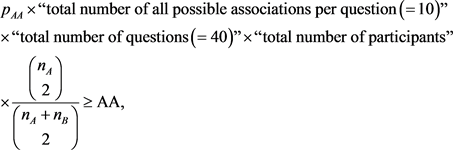
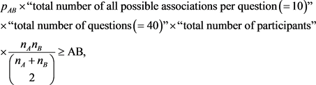
where AA, AB and BB are the numbers of answered pairs in the experiment connecting both two words in Group A, between one word in Group A and the other in Group B, and both two words in Group B, respectively.

Depending on the requirement (2) in Subsection 2.1 for experiments, “hidden” associations, which may exist, cannot be counted. Thus we only have such inequalities stated in the above.

Applying “total number of participants” = 5, , and in Table 1 to Claim 3.7, we can obtain

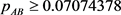and (21)

Here we can also get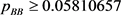, which does not contradict the value obtained by the actual experiment. By (21) and (17) with Propositions 3.5, we can obtain

As a further observation, combining Proposition 2.3 and (21), we have the upper bound estimates for and. Actually we can see

(22)

Similarly, we have

(23)

Consequently, by the experiment in (Takahashi & Tanaka, in preparation), we have

and

for students.

On the other hand, for adults, no such significant difference can be found between mean hit rate in Group A + B and that in Group B: t = −0.48995 and p-value = 0.6244. Refer to Table 1 and (Takahashi & Tanaka, in preparation). Thus we cannot expect or holds. Let us discuss the densities for adults by the same arguments as in the above. Here, , and, Thus we have, by (11) and (15),

and. (24)

Furthermore we have

Next Applying “total number of participants” = 5, , and in Table 1 to Claim 3.3.1, we can obtain

and (25)

Here we can also get, which does not contradict the value obtained by the actual experiment. Obviously, by (25) and (24) as far, we cannot conclude whether

or

holds; in fact, our intuition in (Takahashi & Tanaka, in preparation; Tanaka & Takahashi, 2019) is that and hold approximately, which does not contradict the discussion above.

Again, by the same argument as in the case for students with the results for adults in (Takahashi & Tanaka, in preparation), we consequently have

and

for adults.

3.3.2. In Further Study of Tanaka and Takahashi

In a further study of Tanaka and Takahashi (Tanaka & Takahashi, 2019), for 32-students, there was also a significant difference between mean hit rate in Group A + B and that in Group B via classical Welch t-test: t = 4.4578 and p-value = 8.637e-06 < 0.00001. Also in this case, we will show and by the same arguments as in the previous subsection 3.3.1.

Let us calculate in Proposition 3.3 and in Proposition 3.5. Referring to Table 2, we find, , and . Thus we have, by (11) and (15),

and. (26)

In this case, we see and

and,

which does not satisfy (12) in Proposition 3.4.

Now applying “total number of participants” = 32, , and in Table 2 to Claim 3.7, we can obtain

and (27)

here we can also get, which does not contradict the value obtained by the actual experiment. By (27) and (26) with Propositions 3.3 and 3.5, we can obtain

and.

Again, by the same argument as in the previous subsection, we consequently have

and

for this experiment.

3.4. Modelling towards Actual Experiments

Assumption 3.8. (The Lorentz-Berthelot rules) We assume the relation among three densities as

(28)

where and implies the density (probability) connecting two words in Group A, Group B and between Group A and B, respectively.

Let us give a brief explanation of Assumption 3.8 stated above. The relation (28) corresponds to the Lorentz-Berthelot rules or the Berthelot rule, which is well known as one of basic combining rules in computational chemistry and molecular dynamics. In our context, it is natural to consider every word in Group A and B corresponds to a particle of two categories of identical particles A and B, respectively. Therefore three densities and can be also considered as the interaction force within A, B and between A and B, respectively. In this sense, it is natural to give the relation (28) among and by the Berthelot rule in our setting. We should remark that we put in the experiments of Takahashi and Tanaka. In addition, once densities and are obtained by actual experiments, we can calculate other densities and by the relations (28) and (4). The explicit expressions of and in terms of, , and, which are somewhat complicated forms, can be seen in Subsection A5 in Appendix. Calculated results are shown concretely in Table 3 and Table 4 in Subsections 3.4.1 and 3.4.2, respectively.

As stated before Claim 3.7, we should take care in dealing associated pairs in the participants’ answers. The requirement asked for all participants, which is suitable in the actual experiments discussed in Subsection 2.1, is that the participants must indicate at most one-pair with association per question. By virtue of this requirement, when two words are chosen as one pair in some item, we cannot judge whether it may be only one pair in this item, or it may be stronger one pair than other one or more pairs, or it may be one pair in a triangle or more complicated subgraph. In other words, we cannot know how strong the answered pair is, and whether other hidden pairs are within Group A, Group B, or, between Group A and Group B. Namely, this requirement might break the structure of associations which may exist potentially in answering. For these

Table 3. Results summary for (Takahashi & Tanaka, in preparation).

Table 4. Results summary for (Tanaka & Takahashi, 2019).

reasons, it is dangerous to investigate the details among all the answered “associations”, nevertheless they have fruitful information. Let us illustrate an example using the concrete density in the result for student in (Takahashi & Tanaka, in preparation); refer to also Table 1. Here we should remark the following holds:

Then there is expected to be 45.96, derived from, associations

for one participant in average, but the number of answered association, which are asked to be answered as one association per question, is 28.2, derived from 141/5, per participant in average. The difference per participant between them, about 18-associations, are considered to be hidden due to the requirement in one person’s answering. On the other hand, the impression for almost all participants is that almost all answered association were unique and there were three questions at most having two or three associations (Takahashi & Tanaka, in preparation; Tanaka & Takahashi, 2019). The interpretation about this difference between the measured quantities and their impressions is a further problem for (psycho)linguistics.

Although there exist some problems like stated above, it is plausible to consider the ratio among three types of answered associations, AA:AB:BB, as a “criterion” for the ratio among three types of associations which might be appeared in minds. Moreover, each expected number of pairs per question derived from our experiments (cf. Table 1 and Table 2) is at most 1.5 fortunately; this suggests the hidden association are somewhat small. In any case, the ratio of pairs within Group A, Group B and between Group A and Group B among all the answered associations should be treated very carefully.

Under such discussion above, let us compare the ratio AA:AB:BB with two types of ratios: one is the ratio, which does not contain any densities and another is the ratio, which contains densities derived from our experiments and modelling. Their details are as follows.

1) The ratio among the numbers of pairs of both in Group A, between Group A and Group B and in Group B becomes

(29)

by Equation (38) in Appendix. For details, refer to Subsection A2 in Appendix; here we write for in Subsection A2. In this case, we do not consider any densities. Since and in all experiments we treat, we have the normalized ratio as

(30)

2) Considering the densities and, which are calculated via Claim 5.5, and derived from the experiments, we define the ratio as

(31)

If we assume that all densities would be equal, in (31), then we have (29).

3.4.1. For Preliminary Study of Takahashi and Tanaka

From experiments (cf. Table 1), we have the total numbers of answered pairs connecting two words in Group A, between Group A and B, and in Group B are follows:

Students: AA = 30, AB = 67, BB = 44; AA + AB + BB = 141 (total 200 items);

Adults: AA = 32, AB = 66, BB = 58; AA + AB + BB = 156 (total 200 items).

Also we recall that and for students; and for adults.

We can see a slight difference of the ratio AA:AB:BB of student for the ratio among and (without their densities); in addition, we can see a slight difference of adults for the ratio among and (with their densities). Here we use a statistical programming language R (R Core Team, 2019) for numerical calculations and the chi-square test. See Table 3.

On the other hand, we can see no significant difference of the ratio AA:AB:BB of student for the ratio among and (with their densities) and that of adults for the ratio and (without their densities).

Therefore we may say the density of adults would be uniform in all the words A and B and our densities derived in our modelling are fit on the data for students in the sense that there exists no significant difference from the ratio among AA, AB and BB.

3.4.2. For Further Study of Tanaka and Takahashi

From experiments (cf. Table 2), we have the total numbers of answered pairs connecting two words in Group A, between Group A and B, and in Group B are as follows:

Also we recall that and.

We derived, from the chi-square test, a significant difference of the ratio AA:AB:BB for the ratio among and in 1). On the other hand, we cannot derive a significant difference of the ratio AA:AB:BB for the ratio among and in 2). See Table 4.

Then, combining with the discussion in the previous subsection 3.4.1, we may say our densities for students in our modelling are fit on the data in the sense there exists no significant difference from the ratio among AA, AB and BB.

Consequently, we presume the Lorentz-Berthelot rules in (28) can be applied to the densities in the mental lexicon network of L2 “young” learners, which is considered to be in the process of evolution; for L2 “matured” learners, their mental lexicon network are considered to be almost completed. For details, these topics should be discussed in the context of linguistics or psychology.

4. Concluding Remarks

The main topics discussed in (Takahashi & Tanaka, in preparation; Tanaka & Takahashi, 2019) are explorations of the structure of the mental lexicon of L2 learners’ in the context of (psycho)linguistics. Though a concept of random graph is introduced and applied essentially, only rough ideas derived mathematically are provided and details are omitted. Thus one of main topics in this paper is to give the explicit formulae and their proofs, which are seen in Section 3.3 and in Section A4, respectively. In addition, we propose a kind of modelling for actual experiments in (Takahashi & Tanaka, in preparation; Tanaka & Takahashi, 2019). We know that there exist many types of restriction in doing actual experiments although we always want to get sufficiently many kinds of data. In the sense that much information is derived by the actually obtained data so far, our proposal may be useful. For example, the “hit rate” in the n-word task brings us the “density” via a generalized form of Proposition 2.1 and Remark 2.4.

Here we discussed almost all topics in terms of mathematics, but many results should be interpreted and discussed in the context of (psycho)linguistics (cf. Takahashi & Tanaka, in preparation; Tanaka & Takahashi, 2019), that is, we believe many fruitful and further studies are brought.

Acknowledgements

The authors wish to thank the anonymous reviewers for comments on earlier version of this paper. In addition, they wish to thank Professor Jenny Zhang, Managing Editor, and the staff members of OJML for their invaluable editing task. The authors also would like to express their sincere gratitude to Professors Hiroshi OGURA, Etsuo SEGAWA and Yusuke YOSHIKAWA for their helpful suggestions. YuH’s work was supported in part by Japan Society for the Promotion of Science Grant-in-Aid for Scientific Research Grant Numbers (C)25400208, (A)15H02055 and (C)18K03401. MT acknowledges financial supports from the Grant-in-Aid for Scientific Research (C) Japan Society for the Promotion of Science (Grant Number 17K02762).

Appendix

A1. Flow of Actual Experiment-Five-Word Task

1) INPUT: Participant looks at 5 words per one question. See also FigureA1.

2) Example of possibilities in a participant’s mind: total number of possibilities is 1024(=2¹⁰). See also FigureA2.

3) Required condition: Choose the at most one association (or two words) with the strongest link, even if two or more associations exist.

4) OUTPUT: Answer one association of two words or no association. See also FigureA3.

5) Go to the next question, that is, return to 1) in the next one.

A2. Counting and Probability

Let and be the numbers of words in Group A and Group B, respectively. The event that both two associated words belong to Group A in a given word set consisting of five words selected randomly from Group A + B is denoted by. Let us show the probability can be given as

Let X be the random variable such that the number of words belong to Group A in a word set, that is, randomly selected five words. Then we have the probability as

Figure A1. Example of a questionnaire in Step (1).

Figure A2. Example of Step (2): latent patterns of association.

Figure A3. Example of Step (3): answer.

Thus can be expressed by

(32)

Here we remark the following relation: for positive integers,

(33)

Thus we can express the numerator and denominator in (32) as follows by putting and in (33), respectively:

and.

Then we obtain

(34)

where we use the total mass for the hypergeometric distribution is equal to 1:

(35)

The argument stated above similarly gives

and (36)

where and are probabilities such that both two associated words belong to Group B and one word belongs to Group A and the other does to Group B in a given word set consisting of five words selected randomly from Group A + B, respectively.

Then the ratio of numbers of association pair that both two words are in Group A, one word is in Group A and the other in Group B or both two words are in Group B is estimated as

(37)

In experiments in Takahashi and Tanaka (Takahashi & Tanaka, in preparation; Tanaka & Takahashi, 2019), we have approximately the normalized ratio

(38)

since and.

A3. Mean Field Theoretic Approximation

If we consider the mental lexicon network model in which a unique probability of association occurring p, then the relations (1) and (2) hold and its “density” coincides with p via the “hit rate” derived from word association tasks. However, in the setting where two or more kinds of densities, the hit rate from “k-word task” () is estimated in another expression. Let us show it in our model exhibited in Section 2.2.2. The “hit rate” can be expressed explicitly as follows:

(39)

where we set for. In the above, the probability from (2) may be said to be the averaged “probability” in the whole set Group A + B, that is, two bodies system of Group A and Group B with, and is translated into one body system Group A + B with. We should remark that, which is expressed by, and, cannot coincide with the ratio of number of edges in G as is shown in (3), in general, and that the relation (39) coincides with the general assumption (4) when. Referring to (35) in Section A2, we obtain

(40)

where implies the probability of any association not occurring in “k words” selected randomly, which consist of “words” in Group A and “words” in Group B. Let p be and p be sufficiently small. Then, the left hand side of (40) is

(41)

and the right hand side of (40) is

(42)

where is the asymptotic little-o notation. Referring to (35) again in Section A2, we obtain

(43)

Moreover, referring to (33) in Section A2, we can see that the left hand side of (43) is

(44)

and the right hand side of (43) is

(45)

where we set if. Thanks to (35) again in Section A2, (45) can be simplified as

(46)

Consequently we have

(47)

which implies the exact relation (40) in the “ -word task” for can be well approximated by the relation (4) if all densities are sufficiently small. This is a reason why the relation (4) is set as the plausible general assumption throughout this paper. However, if some density in the networks is not small, the relation (40) may no longer be approximated by the relation (4), that is, the averaged probability may be quite different from the “density” in the network, the ratio of number of edges in a graph G as is shown in (3). See an example in Section A6.2; see also (Meara, 2007).

A4. Proofs of Inequalities for Our Estimation

Proof of Proposition 3.3. Let us evaluate. By Definition 3.1 and Proposition 2.3, we have

Therefore we obtain if and only if

(48)

If the inequality (12) holds, then; thus holds for any. Let us show the monotonically decreasing of the right hand side of the inequality (12), that is,

Then we have, by remarking the relation,

(49)

which implies that this monotonically decreases as increases and tends to 1 as. Thus the proof is completed.

Proof of Proposition 3.5. Let us evaluate. By Definition 3.4 and Proposition 2.3, we have

Therefore we obtain if and only if

(50)

If the inequality (16) holds, then; thus holds for any. The remaining part is trivial from the form of the right hand side of the inequality (16). Thus the proof is completed.

Proof of Corollary 3.6. Let us recall Equation (11):

In addition, we can express in Equation (15) as

Then we have, by remarking the relation,

(51)

which completes the proof.

A5. Exact Expressions of Densities under Assumption 3.8

Claim 5.1. Let and be positive integers. Moreover let, , and be probabilities. Under the assumption that (4) and (28) hold, we have

(52)

(53)

for given and.

Proof. It follows from (4) and (28) that

(54)

Let us consider the following function on x:

(55)

Here, remarking (4), we easily see that

and that

if and only if. In addition, again remarking (4), we easily see that ; thus there exists a unique solution, which corresponds to, such that. Solving the quadratic equation, we obtain

(56)

Simplifying (56) leads to

(57)

Combining (57) with

and,

we can get the desired expressions (52) and (53) in Claim 5.1.

A6. Mathematical Interpretations on Some Models in (Wilks, Meara, & Wolter, 2005); (Meara, 2007)

A6.1. For a Model in Wilks, Meara, & Wolter 2005

In Wilks, Meara, & Wolter (2005), they modified the original model in Wilks & Meara (2002) by considering some association “indirectly” linked between two words. In terms of a random digraph, two words x and y are associated if or in the original model; in addition, they consider two words and are also associated “indirectly” if there exists a word such that and. In such a model, referring to Remark 2.4 for random digraphs, we can easily find, for a randomly selected n-words experiment,

(58)

Here we should remark that the values and imply the probabilities of no direct association occurring within a randomly selected n-words and no indirect association occurring in a randomly selected n-words via some word z outside n-words, where the total number of such words are, respectively. Following (Wilks, Meara, & Wolter, 2005), we put and in (58); we have

(59)

where we put and k is the “number of links per word”, in other words, the regularity of outer degree in digraph; this formula (59) almost recovers the results of simulations in Table3 in (Wilks, Meara, & Wolter, 2005). See TableA1.

Table A1. Outputs of (59) for ().

A6.2. For a Model in Meara (2007)

In Meara (2007), as a kind of small world model, the following random digraph model is introduced: 1) 1000 words are grouped into 20 cluster, each consisting of 50 words; 2) within these clusters, every word has random k-out-degree (); 3) among these clusters, we give additional 50 arcs. For details, see Section III.2 in (Meara, 2007). In the sense of the probability of arc occurring, it is obvious that within every cluster is quite denser than among clusters; this implies every cluster is almost isolated. For such a model, the results of “hit rates” in the task of five randomly selected words under the computer simulations are given. Now let us interpret these results in our context and methods. First we divide into 7 cases based on the number and type of clusters to which selected 5 words belong: case (1, 1, 1, 1, 1), case (2, 1, 1, 1), case (2, 2, 1), case (3, 1, 1), case (3, 2), case (4, 1), case (5).

1) For case (1, 1, 1, 1, 1): This implies there exist 5 clusters such that each of them includes just one word in randomly selected 5 words. Then, considering “direct” and “indirect” associations by the similar way to that in the previous subsection, we can obtain the probability of association occurring within 5 words in this case that

(60)

here any association occurs among clusters only and never occurs within each cluster in this case.

2) For case (2, 1, 1, 1): This implies there exist 4 clusters such that just one of them includes two words and each of three others does just one word. Then, considering “direct” and “indirect” associations within cluster and among clusters, we can obtain the probability of association occurring within 5 words in this case that

(61)

3) For case (2, 2, 1): This implies there exist 3 clusters such that one of them includes one word and each of two others does just two words. Similarly we have

(62)

4) For case (3, 1, 1): This implies there exist 3 clusters such that one of them includes 3 words and each of two others does just one words. Similarly we have

(63)

5) For case (3, 2): This implies there exist 2 clusters such that one of them includes 3 words and another does just 2 words. Similarly we have

(64)

6) For case (4, 1): This implies there exist 2 clusters such that one of them includes 4 words and another does just 1 word. Similarly we have

(65)

7) For case (5): This implies there exists just one cluster including 5 words selected randomly. Similarly we have

(66)

Here any association occurs within one cluster only and never occurs among clusters in this case.

Thus we find, combining all formulae stated above,

(67)

for a randomly selected 5-words experiment. This is valid for general probabilities q within each cluster and r among clusters. Furthermore it is obvious that the function (67) on q and r, both of which are defined on, is monotonically increasing as q or r increases. Incidentally, we remark that, if every cluster is completely isolated, equivalently, then the “hit rate” takes values in . On the other hand, the “hit rate” is bounded above and below for a fixed. For example, if, then the “hit rate” takes values in; these bounds are almost same as those in the case where, respectively, thus we may say every cluster is almost isolated even if. Similarly, for a fixed, the “hit rate” is also bounded; if, then the “hit rate” takes values in .

Now, in order to compare with the results of simulations in (Meara, 2007), let us put and and observe every output value of (67) for. We immediately find our TableA2 almost recovers the results of simulations in Figure 7 in Meara (2007).

We may recover other results in simulation by similar discussion.

Table A2. Outputs of (67) for () and.

NOTES

*Dedicated to the memory of Professor Yoichiro Takahashi.

Conflicts of Interest

The authors declare no conflicts of interest regarding the publication of this paper.

References

[1]	Aitchison, J. (1987, 2012). Words in the Mind: An Introduction to the Mental Lexicon (1st ed. 1987, 4th ed. 2012). Hoboken, NJ: Wiley.
[2]	Barabási, A. L. (2009). Scale-Free Networks: A Decade and Beyond. Science, 325, 412-413. https://doi.org/10.1126/science.1173299
[3]	Barabási, A. L., & Albert, R. (1999). Emergence of Scaling in Random Networks. Science, 286, 509-512. https://doi.org/10.1126/science.286.5439.509
[4]	Boyd, R. (1993). Metaphor and Theory Change. In A. Ortony (Ed.), Metaphor and Thought (2nd ed.). Cambridge: Cambridge University Press.
[5]	Csardi, G., & Nepusz, T. (2006). The Igraph Software Package for Complex Network Research. InterJournal, Complex Systems, 1695, 1-9. http://igraph.org
[6]	Dörnyei, Z., & Taguchi, T. (2010). Questionnaires in Second Language Research: Construction, Administration, and Processing. New York: Routledge. https://doi.org/10.4324/9780203864739
[7]	Erdös, P., & Rényi, A. (1959). On Random Graphs I. Publicationes Mathematicae Debrecen, 6, 290-297.
[8]	Gaskell, G. (2009). Oxford Handbook of Psycholinguistics. Oxford: Oxford University Press.
[9]	Gillham, B. (2008). Developing a Questionnaire (2nd ed.). London: Continuum.
[10]	Gruenenfelder, T. M., & Mueller, S. T. (2007). Power Law Degree Distributions Can Fit Averages of Non-Power Law Distributions. Research on Spoken Language Processing Progress Report No. 28, Bloomington, IN: Indiana University.
[11]	Gruenenfelder, T. M., & Pisoni, D. B. (2005). Modeling the Mental Lexicon as a Complex System: Some Preliminary Results Using Graph Theoretic Measures. Research on Spoken Language Processing Progress Report No. 27, Bloomington, IN: Indiana University.
[12]	Gruenenfelder, T. M., & Pisoni, D. B. (2009). The Lexical Restructuring Hypothesis and Graph Theoretic Analyses of Networks Based on Random Lexicons. Journal of Speech, Language, and Hearing Research, 52, 596-609. https://doi.org/10.1044/1092-4388(2009/08-0004)
[13]	Harley, T. A. (2010). Talking the Talk: Language, Psychology and Science. Hove: Psychology Press. https://doi.org/10.4324/9780203853030
[14]	JACET (2016). The New JACET List of 8000 Basic Words. Tokyo: Kirhara-Shoten.
[15]	Kiss, G. (1968). Words, Associations and Networks. Journal of Verbal Learning and Verbal Behaviour, 7, 707-713. https://doi.org/10.1016/S0022-5371(68)80130-6
[16]	Marcus, G. (2001). The Algebraic Mind: Integrating Connectionism and Cognitive Science. Cambridge, MA: MIT Press. https://doi.org/10.7551/mitpress/1187.001.0001
[17]	Meara, P. (1992). Network Structures and Vocabulary Acquisition in a Foreign Language. In P. Arnaud, & H. Bejoint (Eds.), Vocabulary and Applied Linguistics (pp. 62-70). New York: Macmillan. https://doi.org/10.1007/978-1-349-12396-4_6
[18]	Meara, P. (2007). Simulating Word Associations in an L2: Approaches to Lexical Organisation. International Journal of English Studies, 7, 1-20.
[19]	R Core Team (2019). R: A Language and Environment for Statistical Computing. https://www.R-project.org
[20]	Rapaport, A., Livant, W. P., & Boyd, J. (1966). A Study of Lexical Graphs. Foundations of Language, 2, 338-376.
[21]	Schur, E. (2007). Insights into the Structure of L1 and L2 Vocabulary Networks: Intimations of Small Worlds. In H. Daller, J. Milton, & J. Treffers-Daller (Eds.), Modelling and Assessing Vocabulary Knowledge (pp. 182-204). Cambridge: Cambridge University Press. https://doi.org/10.1017/CBO9780511667268.013
[22]	Scott, J. (1991). Social Network Analysis: A Handbook. London: Sage.
[23]	Stella, M., Beckage, N. M., Brede, M., & De Domenico, M. (2018). Multiplex Model of Mental Lexicon Reveals Explosive Learning in Humans. Scientific Reports, 8, Article No. 2259. https://doi.org/10.1038/s41598-018-20730-5
[24]	Takahashi, R., & Tanaka, M. (in preparation). An Exploration of Density in L2 Word Association Networks in the Mental Lexicon of Japanese Learners of English.
[25]	Tanaka, M., & Takahashi, R. (2019). The Dynamic Characteristics in the L2 Mental Lexicon (pp. 61-66). IEICE Tech. Rep. 119, No. 151, TL2019-23.
[26]	Vitevitch, M. (2008). What Can Graph Theory Tell Us about Word Learning and Lexical Retrieval? Journal of Speech, Language, and Hearing Research, 51, 408-422. https://doi.org/10.1044/1092-4388(2008/030)
[27]	Vitevitch, M. S., Goldstein, R., Siew, C. S. Q., & Castro, N. (2014). Using Complex Networks to Understand the Mental Lexicon. In Yearbook of the Poznan Linguistic Meeting (Vol. 1, pp. 119-138). Berlin: De Gruyter Open. https://doi.org/10.1515/yplm-2015-0007
[28]	Wilks, C., & Meara, P. (2002). Untangling Word Webs: Graph Theory and the Notion of Density in Second Language Word Association Networks. Second Language Research, 18, 303-324. https://doi.org/10.1191/0267658302sr203oa
[29]	Wilks, C., & Meara, P. (2007). Implementing Graph Theory Approaches to the Exploration of Density and Structure in L1 and L2 Word Association Networks. In Modelling and Assessing Vocabulary Knowledge (pp. 167-181). Cambridge: Cambridge University Press.
[30]	Wilks, C., Meara, P., & Wolter, B. (2005). A Further Note on Simulating Word Association Behaviour in a Second Language. Second Language Research, 21, 359-372. https://doi.org/10.1191/0267658305sr251oa