Solution of a Nonlinear Delay Differential Equation Using Adomian Decomposition Method with Accelerated Formula of Adomian Polynomial

Abstract

The aim of this paper is to apply Adomian decomposition method (ADM) for solving some classes of nonlinear delay differential equations (NDDEs) with accelerated Adomian polynomial called El-kalla polynomial proposed by El-kalla [1]. The main advantages of El-kalla polynomials can be summarized in the following main three points: 1) El-kalla polynomials are recursive and do not have derivative terms so, El-kalla formula is easy in programming and save much time on the same processor compared with the traditional Adomian polynomials formula; 2) Solution using El-Kalla polynomials converges faster than the traditional Adomian polynomials; 3) El-Kalla polynomials used directly in estimating the maximum absolute truncated error of the series solution. Some convergence remarks are studied and some numerical examples are solved using the Adomian decomposition method using the two polynomials (Adomian polynomial and El-kalla polynomial). In all applied cases, we obtained an excellent performance that may lead to a promising approach for many applications.

Share and Cite:

El-Kalla, I. , Elgaber, K. , Elmahdy, A. and Sayed, A. (2019) Solution of a Nonlinear Delay Differential Equation Using Adomian Decomposition Method with Accelerated Formula of Adomian Polynomial. American Journal of Computational Mathematics, 9, 221-233. doi: 10.4236/ajcm.2019.94017.

1. Introduction

Delay differential equations are frequently used to model real life phenomena in various fields such as mechanics, computer science, biology and chemistry. Some of the recent studies involving delay differential equations include topics as varied as epidemic models that describe the fraction of a population infected by a virus [2]. In recent years, many papers were devoted to the problem of approximate solution of the NDDEs [3] [4] [5] [6] [7]. The Adomian decomposition method has been shown [8] [9] [10] to solve effectively, easily, and accurately a large class of linear, nonlinear, ordinary and partial differential equations with approximate solutions which converge rapidly to accurate solutions. Adomian decomposition method is a semi-analytical method that was developed from 1970s to 1990s by George Adomian, chair of the center for applied mathematics at the University of Georgia in the USA. Also, Wazwaz discussed the solutions to boundary value problems of higher order by the modified decomposition method [11]. Also, Al-Mazmumy and Al-Malki discussed Some Modifications of Adomian Decomposition Methods for Nonlinear Partial Differential Equations [12]. The basic motivation of this work is to compare between the solution of the NDDEs by the Adomian decomposition method using El-kalla polynomial and Adomian polynomial with the exact solution. First, we will talk about the Adomian decomposition method, then we talk about the formulas that calculate the two polynomials, then we will talk about the Convergence Remarks of the method, then we solve some examples to show the importance of the new accelerated formula called El-kalla polynomial.

2. The Method

L u ( x ) = h ( x ) + f ( x , u ( x ) , g ( u ( x ) ) ) , 0 x 1 (1)

where L = d n d x n is the highest derivative respect to the variable x,

f ( x , u ( x ) , g ( u ( x ) ) ) is the nonlinear term and h ( x ) is any other terms. We will separate the highest derivative on the left side of the equation. Then we take L 1 to both sides, where L 1 is integration from 0 to x. After integration the nonlinear term will be the Adomian polynomial term or El-kalla polynomial such that:

u ( x ) = u ( 0 ) + L 1 h ( x ) + L 1 ( A n ) . (2)

Then Adomian solution assumes that:

u ( x ) = n = 0 u n = u 0 + u 1 + u 2 + u 3 + (3)

u 0 = u ( 0 ) + L 1 h ( x ) u n + 1 = L 1 ( A n ) where n = 0 , 1 , 2 , 3 , (4)

After making the integration we get the solution, where A 0 , A 1 , A 2 , are Adomian polynomials, or we can use the new El-kalla polynomials A ¯ 0 , A ¯ 1 , A ¯ 2 ,

A n = 1 n ! ( d n d ƛ n [ N ( i = 0 n ƛ i u i ) ] ) ƛ = 0 , (5)

where N ( u i ) is the nonlinear term.

A ¯ n = f ( S n ) i = 0 n 1 A ¯ i , (6)

where A ¯ n , are El-kalla polynomials, A ¯ 0 , A ¯ 1 , A ¯ 2 , , f ( S n ) is the substitution of the summation of dependent variable in the nonlinear term.

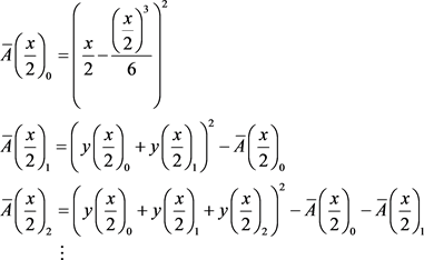
For example the Adomian polynomials & El-Kalla polynomials of the nonlinear term y 2 are showen in Table 1 we can see that the terms using El-Kalla polynomials appear faster than Adomian polynomial.

Also the nonlinear term y 3 the Adomian polynomials & El-kalla polynomials are shown in Table 2 we can see that the terms of El-kalla polynomials appear faster than Adomian polynomials.

3. Convergence Remarks

Many authors discussed Convergence of the Adomian decomposition method. For example, K. Abbaoui and Y. Cherruault [13] [14] [15] proved the convergence of the Adomian method for differential and operator equations. E. Babolian and J. Biazar, contemplate the order of the convergence of the Adomian method in [16]. Zhang [17] presented a modified Adomian decomposition method to solve a class of nonlinear singular boundary-value problems, which arise as normal model equations in nonlinear conservative systems. Zhu et al. [18] presented a new algorithm for calculating Adomian polynomials for nonlinear operators. Also, many modifications were made to this method by numerous researchers in an attempt to improve the accuracy or extend the applications of this method [19] [20] [21] [22]. Also, El-Kalla polynomial was discussed by El-Kalla In [23] [24] [25] [26] [27], and conclude that El-kalla polynomial was directly used to estimate the maximum absolute truncated error of the Adomian series solution which cannot be estimated using the traditional polynomials.

Table 1. Adomian polynomials and El-Kalla polynomials of the nonlinear term y 2 .

Table 2. Adomian polynomials and El-kalla polynomials of the nonlinear term y 3 .

4. Numerical Examples

4.1. Example 1

Consider the nonlinear delay differential equation:

d y ( x ) d x = 1 2 [ y ( x 2 ) ] 2 , y ( 0 ) = 0 , 0 x 1 (7)

We will solve this problem using Adomian decomposition method using Adomian polynomials and El-kalla polynomials.

4.1.1. Solution by Using Adomian Polynomials

Let, the solution

y = i = 0 y i = y 0 + y 1 + y 2 + , (8)

d y ( x ) d x = 1 2 [ y ( x 2 ) ] 2 (9)

Make integration of both sides from 0 to x, we get:

y ( x ) = x 0 x 2 [ y ( x 2 ) ] 2 d x (10)

y ( x ) 0 + y ( x ) 1 + y ( x ) 2 + = x 2 0 x [ A ( x 2 ) 0 + A ( x 2 ) 1 + A ( x 2 ) 2 + ] d x (11)

y ( x ) 0 = x

y ( x ) 1 = 2 0 x A ( x 2 ) 0 d x

y ( x ) 2 = 2 0 x A ( x 2 ) 1 d x

y ( x ) 3 = 2 0 x A ( x 2 ) 2 d x (12)

where the nonlinear term is [ y ( x 2 ) ] 2 , we calculate A ( x 2 ) 0 , A ( x 2 ) 1 , A ( x 2 ) 2 , from the Equation (5),

A ( x 2 ) 0 = ( x 2 ) 2 A ( x 2 ) 1 = x 4 48 A ( x 2 ) 2 = x 6 1440 (13)

y ( x ) 0 = x y ( x ) 1 = x 3 6 y ( x ) 2 = x 5 120 y ( x ) 3 = x 7 5040 (14)

So, the Solution is

y = i = 0 y i = y 0 + y 1 + y 2 + (15)

y = x x 3 6 + x 5 120 x 7 5040 + , (16)

which leads to the closed form solution:

y ( x ) = sin ( x ) , (17)

which equal to the exact solution.

4.1.2. Solution Using El-Kalla Polynomials

The solution is the same as before in Equations (8)-(12) except when we calculate El-kalla polynomials we use Equation (6) as follow.

A ¯ ( x 2 ) 0 = ( x 2 ) 2 A ¯ ( x 2 ) 1 = ( y ( x 2 ) 0 + y ( x 2 ) 1 ) 2 A ¯ ( x 2 ) 0 A ¯ ( x 2 ) 2 = ( y ( x 2 ) 0 + y ( x 2 ) 1 + y ( x 2 ) 2 ) 2 A ¯ ( x 2 ) 0 A ¯ ( x 2 ) 1 (18)

y ( x ) 0 = x y ( x ) 1 = 2 0 x A ¯ ( x 2 ) 0 d x = x 3 6 y ( x ) 2 = 2 0 x A ¯ ( x 2 ) 1 d x = x 5 ( 5 x 2 336 ) 40320 y ( x ) 3 = 2 0 x A ¯ ( x 2 ) 2 d x = x 7 ( 715 x 8 443520 x 6 + 112379904 x 4 ) 5713316492083200 + x 7 ( 15006351360 x 2 + 425097953280 ) 5713316492083200 (19)

The solution is

y = i = 0 y i = y 0 + y 1 + y 2 + (20)

In Table 3, we introduce the absolute relative error (ARE) between the Exact solution and Solution using El-kalla polynomials. Also, (ARE) between the Exact solution and Solution using Adomian polynomials for some values of x in Example 1.

The time elapsed of the program that calculates the solution of Example 1 in Matlab R2014a:

Using Adomian polynomials = 6.3183 seconds;

Using El-kalla polynomials = 5.6548 seconds;

This data calculated by taking six terms of the series solution y = y 0 + y 1 + y 2 + y 3 + y 4 + y 5 in Example 1 (Figures 1-3).

4.2. Example 2

Consider the nonlinear delay differential equation

d 3 y ( x ) d x 3 = 1 + 2 [ y ( x 2 ) ] 2 , y ( 0 ) = 0 , d y d x ( 0 ) = 1 , d 2 y d x 2 ( 0 ) = 0 , 0 x 1 (21)

We will solve this problem using Adomian decomposition method using Adomian polynomials and El-kalla polynomials.

4.2.1. Solution by Using Adomian Polynomials

Let, the solution

y = i = 0 y i = y 0 + y 1 + y 2 + , (22)

d 3 y ( x ) d x 3 = 1 + 2 [ y ( x 2 ) ] 2 (23)

Figure 1. Solution using Adomian polynomials, solution using El-kalla polynomials and Exact solution of d y ( x ) d x = 1 2 [ y ( x 2 ) ] 2 .

Figure 2. The difference between Exact solution and solution using Adomian polynomials of d y ( x ) d x = 1 2 [ y ( x 2 ) ] 2 .

Figure 3. The difference between Exact solution and solution using El-kalla polynomials of d y ( x ) d x = 1 2 [ y ( x 2 ) ] 2 .

Make integration of both sides from 0 to x, we get

d 2 y d x 2 = x + 2 0 x [ y ( x 2 ) ] 2 d x (24)

Make integration of both sides from 0 to x, we get

d y d x = 1 x 2 2 + 2 0 x 0 x [ y ( x 2 ) ] 2 d x d x (25)

Table 3. The absolute relative error (ARE) between the Exact solution and solution using El-kalla polynomials, also between the Exact solution and solution using Adomian polynomials for some values of x in Example 1.

Make integration of both sides from 0 to x, we get

(26)

(27)

(28)

where the nonlinear term is, we calculate from the Equation (5)

(29)

(30)

So, the Solution is

(31)

which leads to the closed form solution

, (32)

which equal to the exact solution.

4.2.2. Solution Using El-Kalla Polynomials

The solution is the same as before in Equations (22)-(28) except when we calculate El-kalla polynomials as follow:

(33)

(34)

The solution is

(35)

In Table 4, we introduce the absolute relative error (ARE) between the Exact solution and Solution using El-kalla polynomials. Also, (ARE) between the Exact solution and Solution using Adomian polynomials for some values of x in Example 2.

The time elapsed of the program that calculate the solution of Example 2 in Matlab R2014a:

Using Adomian polynomials = 11.8629 seconds;

Using El-kalla polynomials = 6.5055 seconds;

This data calculated by taking three terms of the series solution in Example 2 (Figures 4-6).

Figure 4. Solution using Adomian polynomials, solution using El-kalla polynomials and Exact solution of .

Figure 5. The difference between Exact solution and solution using Adomian polynomials of.

Figure 6. The difference between Exact solution and solution using El-kalla polynomials of.

Table 4. The absolute relative error (ARE) between the Exact solution and solution using El-kalla polynomials, also between the Exact solution and solution using Adomian polynomials for some values of x in Example 2.

5. Discussions

From all the previous examples, we extract that the solution of NDDEs by using the Adomian decomposition method with the new polynomial, El-kalla polynomial, which is faster and more accurate than using it with the traditional polynomial called Adomian polynomial. Also the formula that calculates El-kalla polynomial is simple, but the formula that calculates Adomian polynomial has a derivative term that takes time in calculations. It is clear that the time elapsed in the program that calculates the solution using El-kalla polynomial is less than the time elapsed in the program that calculates the solution using Adomian polynomial that means saving time in Matlab R2014a. Also, the maximum absolute relative error between the solution using El-kalla polynomial and the exact solution is less than the maximum absolute relative error between the solution using Adomian polynomial and the exact solution. And thus El-kalla polynomial can be used in solving a wide range of a nonlinear differential equation in many applications.

Conflicts of Interest

The authors declare no conflicts of interest regarding the publication of this paper.

References

[1] El-kalla, I.L. (2007) Error Analysis of Adomian Series Solution to a Class of Nonlinear Differential Equations. Applied Mathematics E-Notes, 7, 214-221.
[2] Zhang and Chen, H. (2010) Block Boundary Value Methods for Delay Differential Equations. Applied Numerical Mathematics, 60, 915-923.
https://doi.org/10.1016/j.apnum.2010.05.001
[3] El-Safty, A., Salim, M.S. and El-Khatib, M.A. (2003) Convergent of the Spline Functions for Delay Dynamic System. International Journal of Computer Mathematics, 80, 509-518.
https://doi.org/10.1080/0020716021000014204
[4] El-Safty, A. (1993) Approximate Solution of the Delay Differential Equation “Y’’ = f(x, y(x), y(α(x))) with Cubic Spline Functions. Bulletin of the Faculty of Science. Assiut University, 22, 67-73.
[5] EI-Safty, A. and Abo-Hasha, S.M. (1990) On the Application of Spline Functions to Initial Value Problem with Retarded Argument. International Journal of Computer Mathematics, 32, 137-179.
https://doi.org/10.1080/00207169008803825
[6] Ibrahim, M.A.-K., EI-Safty, A. and Abo-Hasha, S.M. (1995) 2h-Step Spline Method for the Solution of Delay Differential Equations. Computers & Mathematics with Applications, 29, 1-6.
https://doi.org/10.1016/0898-1221(95)00024-S
[7] Shadia, M. (1992) Numerical Solution of Delay Differential and Neutral Differential Equations Using Spline Methods. PhD Thesis, Assuit University, Assuit.
[8] Adomian, G. (1994) Solving Frontier Problems of Physics: The Decomposition Method. Kluwer Academic Publishers, Boston.
https://doi.org/10.1007/978-94-015-8289-6
[9] Adomian, G. and Rach, R. (1993) Analytic Solution of Nonlinear Boundary-Value Problems in Several Dimensions by Decomposition. Journal of Mathematical Analysis and Applications, 174, 118-137.
https://doi.org/10.1006/jmaa.1993.1105
[10] Ismail, H.N., Raslan, K.R. and Salem, G.S. (2003) Solitary Wave Solutions for the General KdV Equation by Adomian Decomposition Method. Applied Mathematics and Computation, 154, 17-29.
[11] Wazwaz, A.-M. (2000) Approximate Solutions to Boundary Value Problems of Higher Order by the Modified Decomposition Method. Computers & Mathematics with Applications, 40, 679-691.
https://doi.org/10.1016/S0898-1221(00)00187-5
[12] Al-Mazmumy, M. and Al-Malki, H. (2015) Some Modifications of Adomian Decomposition Methods for Nonlinear Partial Differential Equations. International Journal of Research in Agricultural Sciences, 23, 164-173.
[13] Cherruault, Y. and Adomian, G. (1993) Decomposition Methods a New Proof of Convergence. Mathematical and Computer Modelling, 18, 103-106.
https://doi.org/10.1016/0895-7177(93)90233-O
[14] Abbaoui, K. and Cherruault, Y. (1994) Convergence of Adomian’s Method Applied to Differential Equations. Computers & Mathematics with Applications, 28, 103-109.
https://doi.org/10.1016/0898-1221(94)00144-8
[15] Abbaoui, K. and Cherruault, Y. (1994) Convergence of Adomian’s Method Applied to Nonlinear Equations. Mathematical and Computer Modelling, 20, 69-73.
https://doi.org/10.1016/0895-7177(94)00163-4
[16] Babolian, E. and Biazar, J. (2002) On the Order of the Convergence of Adomian Method. Applied Mathematics and Computation, 130, 383-387.
https://doi.org/10.1016/S0096-3003(01)00103-5
[17] Zhang, X. (2005) A Modification of the Adomian Decomposition Method for a Class of Nonlinear Singular Boundary Value Problems. Journal of Computational and Applied Mathematics, 180, 377-389.
https://doi.org/10.1016/j.cam.2004.11.007
[18] Zhu, Y., Chang, Q. and Wu, S. (2005) A New Algorithm for Calculating Adomian Polynomials. Applied Mathematics and Computation, 169, 402-416.
https://doi.org/10.1016/j.amc.2004.09.082
[19] Almazmumy, M., Hendi, F.A., Bakodah, H.O. and Alzumi, H. (2012) Recent Modifications of Adomian Decomposition Method for Initial Value Problem in Ordinary Differential Equations. American Journal of Computational Mathematics, 2, 228-234.
https://doi.org/10.4236/ajcm.2012.23030
[20] Fadugba, S.E., Zelibe, S.C. and Edogbanya, O.H. (2013) On the Adomian Decomposition Method for the Solution of Second Order Ordinary Differential Equations. International Journal of Mathematics and Statistics Studies, 1, 20-29.
[21] Hasan, Y.Q. and Zhu, L.M. (2008) Modified Adomian Decomposition Method for Singular Initial Value Problems in the Second-Order Ordinary Differential Equations. Surveys in Mathematics and Its Applications, 3, 183-193.
[22] Jebari, R., Ghanmi, I. and Boukricha, A. (2013) Adomian Decomposition Method for Solving Nonlinear Heat Equation with Exponential Nonlinearity. International Journal of Mathematical Analysis, 7, 725-734.
https://doi.org/10.12988/ijma.2013.13070
[23] El-Kalla, I.L. (2013) Piece-Wise Continuous Solution to a Class of Nonlinear Boundary Value Problem. Ain Shams Engineering Journal, 4, 325-331.
https://doi.org/10.1016/j.asej.2012.08.011
[24] El-Kalla, I.L., El Mahlawy, A.M. and Botros, M. (2019) A Continuous Solution of Solving a Class of Nonlinear Two Point Boundary Value Problem Using Adomian Decomposition Method. Ain Shams Engineering Journal, 10, 211-216.
https://doi.org/10.1016/j.asej.2018.11.002
[25] El-Kalla, I.L. (2011) Error Estimate of the Series Solution to a Class of Nonlinear Fractional Differential Equations. Communications in Nonlinear Science and Numerical Simulation, 16, 1408-1413.
https://doi.org/10.1016/j.cnsns.2010.05.030
[26] El-Kalla, I.L. (2012) Error Estimates for Series Solutions to a Class of Nonlinear Integral Equations of Mixed Type. Journal of Applied Mathematics and Computing, 38, 341-351.
https://doi.org/10.1007/s12190-011-0482-3
[27] El-Kalla, I.L. (2012) A New Approach for Solving a Class of Nonlinear Integro-Differential Equations. Communications in Nonlinear Science and Numerical Simulation, 17, 4634-4641.
https://doi.org/10.1016/j.cnsns.2012.05.016

Copyright © 2024 by authors and Scientific Research Publishing Inc.

Creative Commons License

This work and the related PDF file are licensed under a Creative Commons Attribution 4.0 International License.