Fundamental Fields as Eigenvectors of the Metric Tensor in a 16-Dimensional Space-Time ()
1. Introduction
In some previous papers [1] [2] [3] we proposed a first tentative approach to field unification based on the usual Kaluza-Klein theory [4] [5] [6] and extension to non-Abelian Yang-Mills fields [7] [8]. Here we develop an alternative way to attack the problem, which appears to be conceptually more satisfactory and elegant. Our proposal is based on the idea of associating each fundamental interaction field with a vector potential which is an eigenvector of the metric tensor of a multidimensional space-time manifold
(n-dimensional “vierbein”). It is relevant to observe that within an n-dimensional space-time, the metric tensor, when represented onto the basis of its eigenvectors, yields a connection involving a 2-index antisymmetric tensor of the same form as a non-Abelian Maxwell tensor which may be related to the fundamental interaction fields in a quite natural way.
Sec. 2 examines such a formulation of general relativity in n space-time dimensions.
Sec. 3 presents a system of field equations involving both Einstein and Maxwell-like equations for the interaction fields.
Sec. 4 is concerned with the problem of confinement of the interaction fields within the observable 4-dimensional space-time and shows that a non-vanishing particles’ rest mass arises thanks to a suitable gauge function which can be related to a scalar boson field (Higgs boson).
Sec. 5 is devoted to a physical interpretation of the results and the conditions to be required in order that all the known fundamental interactions, (gravitational, electro-weak and strong) may be included within the metric and connection. As we will see a 16-dimensional space-time is required to fit the standard model of elementary particles [9] [10].
Consideration on the placement of fermions within the theory will be the subject of the Secs. 6-8, while in Sec. 9 we examine applications to cosmology of the theory.
The last two sections propose a new way to gravity quantization starting from a suitable energy-momentum tensor of the gravitational field. A complete presentation of the theory and much more has been proposed in my book [11].
2. Tensor Representations onto the Basis of the Eigenvectors of the Metric
Let us consider an n-dimensional space-time manifold
, endowed with a symmetric metric g of signature
and a torsionless connection
. In any local frame
a point x is identified in
by its co-ordinates
, with
. As usual
is the observable time and
are space co-ordinates. The non-underlined indices (
) are reserved to the physically observable components, while the underlined Latin ones (
) identify the non-observable extra components. The connection is given by the Christoffel symbols:
(1)
the inverse metric tensor
begin defined, as usual, by the relation:
(2)
2.1. Metric Tensor and Connection Coefficients
The n linearly independent eigenvectors
of the metric tensor fulfill the orthonormality conditions:
(3)
where
. Then:
(4)
provides its representation onto the basis of its eigenvectors. These orthonormal eigenvectors are undetermined by an imaginary exponential factor
which leaves unchanged the real metric tensor components, provided that the complex scalar product
replaces the real product
. This degree of freedom allows periodic wave propagating field solutions (see Sec. 4.1). In the following we will drop the
complex conjugation mark, leaving it as understood, to avoid too heavy notations.
The representation of the connection coefficients relative to the basis of the eigenvectors becomes now:
(5)
with:
(6)
Significantly the connection includes antisymmetric non-Abelian tensors fields and a symmetric non-tensor field
. It is convenient to introduce also the new symbol (reduced connection):
(7)
Then the complete expression of the connection in
writes also:
(8)
Arising of non-Abelian Maxwell-like tensors
within the connection coefficients suggests that the electro-weak and strong interaction fields may be included into the metric tensor in a unified field theory when the space-time dimensionality is greater than four.
2.2. Ricci Tensor
The Ricci tensor:
(9)
is now to be evaluated on the basis of the eigenvectors of the metric. The following auxiliary notations may be useful:
(10)
from which we obtain:
(11)
thanks to the symmetries. Calculations leading to an explicit representation of
in terms of
and their derivatives are very heavy.
But under the covariant Lorentz gauge condition:
(12)
which can be shown to be equivalent to:
(13)
relevant simplifications arise, resulting:
(14)
Then the Ricci tensor assumes the meaningful form:
(15)
where colon (
) denotes here the covariant derivative respect to the reduced connection and the notation:
(16)
has been introduced. It is convenient to represent also:
(17)
where
is arbitrary, at present, adding vanishing contributions to
and
because of antisymmetry. As we will see in Sec. 5 the tensor
introduces a degree of freedom that will play an important role to fit elementary particle current densities. The Riemannian covariant derivatives will be replaced with non-Abelian covariant ones
, when required. Eventually we obtain:
(18)
the trace of which is given by:
(19)
3. Field Equations
If the Lorentz gauge holds, being equivalent to (13), the Einstein field equations become:
(20)
Introducing the new variables:
(21)
and the energy-momentum tensor
of the fields
, defined by:
(22)
we obtain the following system of field equations:
(23)
(24)
Now, if we represent
onto the basis of the vector potentials, as:
(25)
and the current density:
(26)
we arrive at a physically relevant form of the field equations:
(27)
(28)
Thanks to the Lorentz gauge and the symmetries the last Equation (28) results also equivalent to:
(29)
4. Field Confinement and Particle Rest Masses
4.1. Vanishing of Particle Rest Masses in V4
Let us consider the D’Alembertian field equation governing the potential
in absence of currents:
(30)
We separate now the 4-vector components in
, which will be interpreted as related to the physical interaction fields carried by bosons, from the remaining extra components:
(31)
The latter components behave as scalars when observed within
and may be associated with the matter fields governing fermions. The previous equations can be developed as:
(32)
(33)
Physically we need to preserve covariance respect to any transformation of the co-ordinates within
, which are observable, while we may lose covariance respect to transformations involving the extra co-ordinates in the entire
, since the latter are seen as scalars when observed from the physical space-time
. So separate complex solutions are allowed to the 4-vector field Equation (32), i.e.:
(34)
and for each one of the
-scalar Equation (33):
(35)
The distinct wave numbers
(components of a four-vector) and
(scalars for an observer living in
) are allowed to assume different values for each index
, related to the field
. In correspondence to these solutions Equation (32) and Equation (33) may be written as equivalent to Klein-Gordon equations [12] [13] :
(36)
(37)
where:
(38)
The covariance, which is broken in the extra space, while it is preserved in
, allows different rest mass values which will be attributed respectively to boson vectors carrying the fundamental interactions and to fermions characterizing the matter fields. Manifestly a non-vanishing particle rest mass is related to the dependence of the vector potential on the extra co-ordinates
. So the request that the fields
are confined within the physical space-time
so that they depend only on the observable co-ordinates
, is equivalent to impose that the particles associated with those fields have vanishing rest mass:
(39)
4.2. Particle Masses and Scalar Boson Gauge Fields
Now we will show how non-vanishing particle rest masses are related to the presence of the n-scalar gauge fields
, which seem to play a role similar to the one of the Higgs scalar boson field (see [14] - [19] ). But here a different mass generating “mechanism” is presented, which is based on a suitable gauge choice which is established in order to ensure the confinement of the physically observable fields.
In fact, as it is well known, the n-vector potential
is determined except for a gauge transformation:
(40)
where the n-scalar field
is required to fulfill the D’Alembertian equation:
(41)
so that the Lorentz gauge is preserved. We point out that those scalar fields do not appear in the observable tensors
which are gauge invariant, since:
Then the dependence of
on the extra co-ordinates
does not affect the observables
and cannot be detected by direct observation within the physical space-time
. Introducing now a wave solution for
like:
(42)
into (41) we obtain the Klein-Gordon equation:
(43)
We remark that while a single solution
is required for the covariance of the 4-vector
in
, different solutions:
(44)
are allowed for each value of the index
, to obtain extra components
, each of them being a scalar respect to transformations of the co-ordinates
within
. So different masses:
(45)
arise for the scalar fields contributing respectively to bosons (
) and fermions (
).
If we choose a gauge such that that
depends only on
(so that
), while
(which is not observable in
) may depend also on
, then the gauge transformation (40) implies into (36):
(46)
which in correspondence to the solution(42) for the field
may be written as:
(47)
so preserving the gauge invariance, thanks to (43), resulting:
(48)
We now perform the following transformation of field variables:
(49)
the inverse of which is given by:
(50)
From (50) into (48) we obtain:
(51)
And from (50) into (43) we have:
(52)
It follows:
(53)
After the transformation the fields
are required to fulfill the Klein-Gordon equations:
(54)
(55)
where
, are to be determined. Combination of (54) and (55) with (51) and (53) leads to:
(56)
Then the relations between the masses result to be:
(57)
Non-vanishing particle rest masses arise and are equal to the respective scalar boson masses. Further gauge transformations:
remain possible involving only the observable co-ordinates
, while the gauge is fixed in the extra space-time. The same procedure can be implemented also respect to the extra components
, obtaining the rest masses:
(58)
which will be related to the fermions (leptons and quarks) as we will show in the next section. We emphasize that the gauge fields
may be related to only one scalar field
, according to the relation:
(59)
where
are coupling constants of the vector potentials with a single scalar boson field, for which the solution:
(60)
fulfills the Klein-Gordon field equation:
(61)
Then it results:
(62)
And being
, we obtain:
(63)
Then the masses of the vector bosons carrying the interaction fields would become:
(64)
being:
(65)
The values of
depend on the coupling constant with the scalar boson of mass M. Similarly the masses of fermions result:
(66)
being:
(67)
and
the coupling constants of the fields
with the scalar field
.
5. Interaction Fields (Bosons)
5.1. Gravitational Field
The present section is concerned with the physical interpretation of the components of the vector potentials. We start considering the free gravitational field in ordinary space-time
.
1)
In ordinary empty space-time, when no extra dimensions are present (standard general relativity) the metric tensor is interpreted, as usual, as a free gravitational field. Therefore its eigenvectors
may be conceived as the vector potentials of the free gravitational field. In fact in this occurrence the metric tensor is given by:
(68)
and the potentials
are clearly responsible of gravitation, according to general relativity. The connection is given by:
(69)
where:
(70)
are the coefficients of the reduced connection. The Ricci tensor has simply the form:
(71)
So the Einstein equations are as usual:
(72)
where no energy-momentum tensor appears, since the whole gravitational field is included into space-time geometry.
But if we represent the Ricci tensor in terms of the reduced connection, which only partially embeds the gravitational field into geometry and leaves part of it as an external field of strength
we have the following field equations, in the Lorentz gauge:
(73)
(74)
The energy-momentum tensor of the non-embedded into geometry contribution to the gravitational field appears:
(75)
together with the gravitational current density:
(76)
More, an equivalent gravitational energy-momentum embedded into geometry may be defined:
(77)
So the field equations for the gravitational field can be written in the equivalent energetic form:
(78)
where:
(79)
2)
When the space-time dimensionality is greater than 4, we still associate the potentials labeled by
, to the gravitational field, while we relate the components of additional potentials
, to the non-gravitational interaction fields. We emphasize that when
each vector potential
includes also the extra components
, because of the increased dimensionality of space-time. So we are led naturally to the following physical interpretation.
- The gravitational field observed within the physical space-time
is described by the
, which are 4-vectors in
.
- The electro-weak and strong interactions are associated with the
, (
), which are also 4-vectors in
.
- The remaining components
, which behave as scalars within the observable space-time
are related to the matter fields, i.e., to fermions (leptons, quarks).
We observe also that the sectors of the potentials of indices
:
(80)
solutions to the corresponding Klein-Gordon field equations:
(81)
may be associated with particles of different rest masses:
(82)
if we allow that the covariance is preserved only in the observable space-time
, while it may be broken in the extra dimensions of the multidimensional space-time
.
We emphasize that all the previous masses
result to be null when the vector fields depend only on
. The non-zero rest masses of fermions associated with the
arise thanks to the contribution of the massive scalar gauge fields
which are allowed to depend also on
. The field equations for the gravitational field in
involve now, beside the terms labeled by
, the new contributions labeled by
, and the correspondent additional energy-momentum tensor. We have:
(83)
(84)
where:
(85)
is the energy-momentum of the non-gravitational Maxwellian fields as they may be observed within the physical space-time
.
A more familiar form of the Einstein equations, which hides the whole gravitational field into geometry is obtained if we write the metric tensor as:
(86)
The connection writes now as:
(87)
where a new partially reduced connection is defined by:
(88)
In this way the gravitational field is entirely hidden into geometry and only the non-gravitational fields contribute to the energy-momentum tensor. The field equations become:
(89)
where:
(90)
are the
components of the new partially reduced Ricci tensor, evaluated respect to the partially reduced connection.
Respect to the usual Einstein equations a new term appears, i.e.:
(91)
Moreover
differs from the expected Ricci tensor
in
, being evaluated respect to
instead of:
(92)
A comparison between the usual Einstein equations in
and (73) is possible if we write:
(93)
where:
(94)
is the usual Ricci tensor in
and:
(95)
The additional contributions
and
could be considered as possible contributions to dark energy and dark matter emergence.
5.2. Electro-Weak Field
In order to describe unified electromagnetic and weak fields we need one Abelian field and three non-Abelian ones. So the indices
will be related to electro-weak interactions and the vector potential components:
(96)
will be interpreted as electro-weak fields. The space-time dimensionality required, is now raised up to
. The electromagnetic and weak interaction fields are mixed in the unified electro-weak theory. So the choice of the physical meaning of these vector potentials
will depend on the standard model representation adopted.
Non-diagonal representation
The non-diagonal representation of the electro-weak field involves the vector fields
,
, the corresponding strength tensor being given by:
(97)
where g is one of the electro-weak coupling constants and
is the Levi-Civita symbol. So we are led to associate the components of each potential
in physical space-time
(
) in the following way:
(98)
Dimensional constants depending on the unit system have been absorbed into the definition of the fields themselves. Then the strength field tensors components result:
(99)
Identifying (97) and (99) we determine the structure constants:
(100)
Diagonal representation
According to the standard model the physical fields:
(101)
are provided by the diagonal representation, which is obtained thanks to a rotation of
of the Weinberg angle, defined by the relation:
(102)
being a second electro-weak coupling constant. So that we have the following alternative way to associate our vector potentials with the electro-weak fields:
(103)
In the diagonal representation the strength tensors are obtained through the inverse rotation:
(104)
when substituted into (97). We have:
(105)
Eventually it results:
(106)
Identifying (106) with (99) we reach:
(107)
and determine the relations for the structure constants:
(108)
In each representation the field equations exhibit the Maxwellian form:
(109)
In terms of the vector potentials the previous equation becomes, in the Lorentz gauge, a Klein-Gordon equation with current density. In Sec. 8 we will examine the current density
.
5.3. Strong Interaction Field
The strong interaction field is carried by massless gluons and we are required to add 8 non-Abelian fields
which we relate to the indices
:
(110)
Therefore
space-time dimensions are needed to describe all the known fundamental interactions.
The strength tensors for strong interactions are:
(111)
where
is a suitable coupling constant and the structure constants, according to the standard model, are given by [9] :
(112)
Identification of (99) with (111) now yields:
(113)
The Maxwellian field equations are now:
(114)
6. Matter Fields (Fermions)
Let us, now, examine in more detail all the 16 components
of the vector potential appearing in the theory.
In the previous sections we interpreted the first 4 components of each potential as related to the fundamental interactions (gravitational, electro-weak and strong).
Here we show how it is possible to interpret the remaining 12 extra components, we have labeled by the index
.
As we have shown, these components are seen as scalar fields by an observer living in the physical space-time
, since they are not affected by the transformations of the co-ordinates
in
.
Until now we considered only interaction fields, carried by vector bosons (gravitons, photons,
and gluons) and nothing was said about fermions (leptons and quarks).
Now we introduce also the 6 leptons (
) and the 6 quarks, (up, down, top, bottom, charm, strange) with their respective anti-particles and left/right chirality.
So we may summarize the physical interpretation of the potential components as follows:
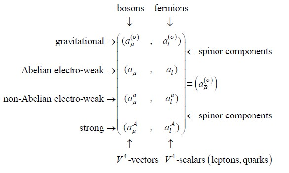
Physical Interpretation of the Field Extra Components
In this subsection we want to show how the 192 extra components of the vector potentials
, may be related to the spinor fields associated with the fermions (leptons and quarks) appearing in the standard model of elementary particle theory.
Each spinor is a set of 4 complex valued functions of the observable co-ordinates
, which are to be provided by the 196 complex functions offered by the extra components of the vector potentials
:
(115)
Each component of
may be evaluated as a linear combination of the
.
The simplest representation is given, of course, by:
(116)
which can always be obtained with a suitable choice of the extra co-ordinates
.
Then we can associate groups of 4 components to the spinors representing the physical elementary fermions, e.g., as:
(117)
where l.h., r.h. denote respectively left-hand and right-hand chirality and red, green, blue the quark color.
According to this scheme a detailed sketch of the physical meaning of all the components of the vector potentials
can be summarized as the following sketch shows.

The index
, running from 4 to 15, it labels 12 spinors corresponding to the 6 leptons
, and to the 6 quarks in dependence on the values of
and 12 more spinors related to the respective anti-particles.
7. Dirac Field Equations
The extra equations which govern fermion fields are given by:
(118)
(119)
(120)
where the energy-momentum tensor includes both the contribution of the interaction fields and the contribution of the gravitational field arising from extra dimensions.
We have:
(121)
(122)
(123)
According to the standard model the covariant derivatives are determined in such a way that the gauge invariance conditions in
are preserved even when a gauge choice is fixed in the extra space-time. Such a choice is always possible because of the degrees of freedom provided by the anti-symmetric tensor
(arbitrary until now). Moreover, thanks to the latter tensor we will be able to obtain also the correct current densities in the r.h.s. of the interaction fields equations.
Now we consider (29), with vanishing currents we have when
:
(124)
Following a scheme like (117) we may replace the latter equation for the potentials
with the second order spinor equation:
(125)
Rest masses and contributions are expected to be hidden into the derivatives respect to the extra co-ordinates, so that (125) identifies with the Klein-Gordon equation:
(126)
which leads to the Dirac equation:
(127)
being the respective rest masses of leptons and quarks, related to the scalar boson mass:
(128)
8. Current Densities
When
, the 4-vector
is to be related to the physical charge current density:
(129)
where the notation
means each kind of charge carried by fermions. Then the identification follows:
(130)
Since
, with
, results to be:
where:
we can determine the until now free term
as:
(131)
9. Cosmological Solution
In this section we examine a cosmological solution to the Einstein field equations in empty extended space-time
. We start generalizing Robertson-Walker metric as follows:
(132)
to which we add the extra components:
(133)
so that the cosmological principle is preserved within the observable space-time
. The
are suitable constants which play a role in order to field quantization [11]. The co-ordinates, as usual, are spherical in
and arbitrary elsewhere:
(134)
In correspondence to this solution the non-vanishing components of the Ricci tensor become:
(135)
(136)
(137)
(138)
the Ricci scalar curvature being:
(139)
Then the only non-vanishing Einstein equations in the empty extended space-time
result:
(140)
(141)
respectively in correspondence to the observable space-time and space-space components. While, for the extra space-space components the field equations are all identical to:
(142)
A first result, arising from existence of the extra dimensions is given by the flatness condition:
(143)
because of compatibility between (141) and (142). The latter compatibility provides a quite natural explanation of the observed flatness of the physical universe, at least in correspondence to this solution. Then only the following equations remain:
(144)
(145)
in which the coefficients
do not appear, while the coefficient
, related to the gravitational field in
, does. Then from (144) one obtains, for positive
(as it is physically observed):
(146)
the integration of which leads to:
(147)
since the empty extended space-time
behaves like a multidimensional De Sitter universe, in which no singularity appears. Equation (145) is also fulfilled by the solution (147). Positive sign in the exponential corresponds to an expanding universe as it is physically observed.
Dark Matter and Dark Energy from Space-Time Extra Dimensions
We remember that the non-vanishing Einstein field equations in
in presence of external matter-energy fields are given by:
(148)
(149)
where matter-energy fields are represented, as usual, as a perfect fluid of energy-momentum tensor:
(150)
being the 4-velocity of the fluid particle, which in a co-moving reference,
being the mass-energy and pressure densities of the fluid. From (144) and (145) we solve:
(151)
which substituted into (148) and (149) leads to:
(152)
(153)
resulting:
(154)
The astonishing result of a negative mass density
provided by (152),
being assumed to be positive, suggests that the cosmological constant, due to the extra space-time dimensions, plays the role of a repulsive gravitational source, which is responsible of universe expansion, together with the positive pressure density
given by (153). So the mass-energy density
and
represent the mass-energy and pressure densities of the empty extended space-time
(vacuum energy and pressure) which are seen as matter contributions by an observer living in
.
The matter term includes:
1) The mass-energy and pressure densities of matter/interaction fields (
) embedded in
space-time geometry, as evaluated respect to the reduced connection
, being equal to the mass-energy and pressure densities of matter/interaction fields as observable in
;
2) The usual
vacuum energy
and a vacuum pressure
densities owed to the cosmological constant (standard dark energy);
3) The residual vacuum energy
and a vacuum pressure
densities owed to the extra space dimensions.
4) The extra mass-energy
and pressure
densities owed to the difference between the usual
connection
and the reduced connection
, previously suggested as hypothetical responsible of dark matter (see Sec 5.1):
(155)
Eventually Equation (148) and Equation (149) may be written equivalently as:
(156)
where:
(157)
Remarkably the total mass-energy and pressure densities:
(158)
are constant and directly proportional to the cosmological constant.
In the following sections we evaluate the mass-energy and pressure contributions of the matter/interaction fields and the dark matter owed to the extra dimensions.
10. Energy-Momentum Tensor of Gravitational Field
In the present section we investigate a way to obtain an interpretation of the Einstein tensor as equivalent to the energy-momentum tensor of gravitational fields (labeled by [G]), in order to be able to quantize the gravitational field itself in a natural manner.
Let us start considering the Einstein field equations in the physical space-time
, in presence of external fields:
(159)
the label [F] denoting the non gravitational contributions to mass-energy. And let us introduce the notation:
(160)
We can interpret in a natural way
as the energy-momentum tensor of the gravitational field and write now the Einstein equations as an energetic balance between the gravitational and non-gravitational fields:
(161)
instead of embedding gravity within the geometry of space-time. From the calculations developed in the previous sections we are able to evaluate
in correspondence to the Robertson-Walker metric. Eventually we have, in presence of more gravitons, labeled by an index p:
(162)
Now we can identify:
(163)
as the energy and pressure densities of the gravitational field as observed in
, which include both visible and dark contributions, pressure being here negative as a consequence of gravitational attraction. Of course the energy and pressure densities of the gravitational field are equal and opposite in sign respect to the mass-energy and pressure densities
given by (152), (153) arising from the non-gravitational fields, so that the balance of gravity and non-gravitational fields is exactly zero.
11. Quantization of the Gravitational Field
Let us now examine the Hamiltonian density of the gravitational field, which is given by the
component of the energy-momentum tensor we have just evaluated. We have, by summation over all the particles:
(164)
the index p labeling each graviton.
Integrating on a space region
of volume V we get the total Hamiltonian of the gravitational field enclosed within this region:
(165)
Note that if
is assumed to be the whole universe at instant t the volume becomes time dependent.
Now we introduce the frequencies
through the relations:
(166)
The square modulus yields (where complex conjugation symbol * has here been reintroduced):
(167)
Then the Hamiltonian becomes:
(168)
Quantization results by replacing the coefficients
with the quantum creation and annihilation operators
, by the correspondence rules:
(169)
The coefficient
being arbitrary it can always be adjusted in such a way to fit the right commutation relations for the operators
:
(170)
thanks to which we obtain:
(171)
which provides also for the gravitational field a quantized Hamiltonian in the usual form as known in q.e.d.
12. Conclusion
We have proposed the guidelines of a possible physical interpretation of a model of unified interaction (boson) and matter (fermion) fields within the geometry of a multidimensional space-time manifold
. We have seen how to identify interaction fields with the vector components
of the eigenvectors
of the metric tensor
in
and the remaining components
with the spinor matter fields. Meaningful consequences of these results have been obtained also in cosmology and a way to quantization of the gravitational field has been examined. All those results have been presented in detail in my book [11].