A Test for Joint Market Efficiency from an Investor’s Perspective

Lakshmi Viswanathan^*, S. Maheswaran, G. Balasubramanian

Institute for Financial Management and Research, Chennai, India.

DOI: 10.4236/tel.[phone]                

Abstract

This paper investigates the cross-country correlation between stock markets and its implications. It does so by introducing a new measure called the Scaled Covariance Difference (SCD), which captures the difference between the covariance of short term returns and longer term returns. This measure has practical implications for portfolio optimization, as well as in testing for the joint efficiency of markets. Our focus in this paper is on including the off-diagonal terms of the variance-covariance matrix in the analysis so as to develop a test for joint market efficiency, unlike the univariate tests for market efficiency which only make use of information along the main diagonal of the variance-covariance matrix. We also demonstrate how to implement the test for joint market efficiency using data on weekly stock returns from the Nifty and S&P 500 indices.

Keywords

Market Efficiency, Variance-Covariance, Cross-Country Correlation, Scaled Covariance Difference

1. Introduction & Literature Review

Stock market efficiency is one of the most fundamental topic of research in finance. In a broad sense, market efficiency depends on the degree to which prices of stocks and other securities reflect all available information in the market. Bachelier [1] argues that the market price reflects past, present and even discounted future events but these events show no apparent relation to price changes. When the price changes are independently, identically and normally distributed, the stock prices follow random walk. The tests of market efficiency are based on testing the random walk hypothesis.

Lo and MacKinley [2] tested the random walk hypothesis by considering the weekly stock market returns. They compared variance estimators derived from data sampled at different frequencies. There are a number of subsequent studies which make use of this variance ratio test to test market efficiency. Huang [3] , Urritia [4] , Smith and Ryoo [5] and Darrat and Zhong [6] tested the efficiency of Asian markets, Latin American markets, European markets and Chinese market respectively using the variance ratio test. All these studies analyze one particular market at a time. Geweke and Feige [7] developed a single joint test of efficiency of several forward foreign exchange markets. They made use of simultaneous equation procedure to test multi-market efficiency. The cointegration literature [8] [9] [10] [11] addresses the concept of markets being collectively efficient. Chan, Gup and Pan [9] examines the cross-country market efficiency hypothesis by using Johansen’s [12] [13] cointegration tests. Forbes and Rigbon [14] explore stock market co-movement during crises by making use of heteroskedasticity biases tests for contagion based on correlation coefficients. Erb, Harvey and Viskanta [15] studied international equity cross-correlations based on a semi-correlation metric that differentiates equity correlations in bull and bear markets.

The variance ratio test using the L-M statistic put forward by Lo and MacKinley [2] applies only to the main diagonal in the variance-covariance matrix. Our focus in this paper is to analyze the off-diagonal covariance terms to develop a test for joint market efficiency. A careful examination of cross-country correlation and its determinants plays an important role in this regard. A change in correlation reflects a change in cross-country covariance or volatility of stock markets. There have been a number of studies that examined the correlation between different stock markets. Kaplanis [16] , King and Wadwani [17] , Koch and Koch [18] , Longin and Slonik [19] , Karolyi and Stulz [20] , Longin and Slonik [21] , Wong, Agarwal and Du [22] are to name a few.

The above-mentioned studies analyze the variance-covariance matrix to examine the cross-country correlation over time. The first contribution of our paper is that we examine the correlation and its determinants of short term returns as well as the long term returns (ranging from 1-week return to 8-week returns) of the US and Indian stock markets over the time period under study. Secondly, rather than using the variance-covariance (VCV) matrix, we observe k-week correlation, scaled covariance and V-ratio. More importantly we introduce the measure, Scaled Covariance Difference (SCD) to check if there exists any significant difference between 1-week covariance and k-week covariance. This measure serves beneficial in portfolio optimization as well as to test the joint efficiency of two markets. In this paper we limit our effort on making use of SCD to develop a joint test of market efficiency from an investor’s perspective.

We consider weekly returns from Nifty and S&P500 index for empirical analysis. What we find is that the factors under study (k-week correlation and k-week scaled covariance) appear more or less flat before and after the global financial crisis. However, the level of these factors has changed subsequent to the crisis. The V-ratio remains insignificant for Nifty and S&P500 across all samples. The SCD remains insignificant for all k-week across all samples. This suggests that the information transmission between markets happens within the same week.

The rest of the paper is organized as follows. Section 2 summarizes the Methodology by explaining the theory (2.1), equations and hypotheses (2.2). Section 3 explains empirical analysis. Section 4 presents empirical results. The 5th section concludes.

2. Methodology

2.1. Theory

First we obtain weekly log returns from stock index X and then generate k-week log returns using the formula given below.

$S{x}_t\left(k\right)={\displaystyle {\sum }_{i=0}^{k-1}{x}_{t-i}},\left[1\le k\le 8\right]$ (1)

For an investor from country A with stock index X, returns from country B with stock index Y_B is:

$Y=\ln \left(1+R_s\right)+\ln \left(1+R_{fx}\right)$

where $R_s=\frac{Y_{Bt}-Y_{B\left(t-1\right)}}{Y_{B\left(t-1\right)}}$ and $R_{fx}=\left(\frac{{\text{Exchange rate}}_t-{\text{Exchange rate}}_{t-1}}{{\text{Exchange rate}}_{t-1}}\right)$

We compute k-week log returns using the following equation.

$S{y}_t\left(k\right)={\displaystyle {\sum }_{i=0}^{k-1}{y}_{t-i}},\left[1\le k\le 8\right]$ (2)

where, $x_t$ is the weekly log return (from stock index X), $y_t$ is the weekly log return (from stock index Y after taking the fluctuations into account), k is the number of weeks to be summed up (as a moving window). That is to say to obtain longer term returns, we add up x_t or y_t (1-week returns) over k-week moving window, such as when k =1, the original series is taken as it is and consists of weekly return data. When k = 2, observations 1 & 2, 2 & 3 etc. are added to form a new series of 2-week returns etc.

We compute the k-week correlation, k-week scaled covariance and k-week V-Ratio using the following formulae.

$k\text{-week correlation}:{\rho }_{x,y}=\frac{\text{Covariance}\left(x_{\left(k,t\right)},y_{\left(k,t\right)}\right)}{{\sigma }_{x_{\left(k,t\right)}}{\sigma }_{y_{\left(k,t\right)}}}$

$k\text{-week Scaled covariance}=\frac{k\text{-week Covariance}\left(x_t,y_t\right)}{k}$

$k\text{-week V-Ratio}=\frac{Var\left(k\text{-week return}\left(x_t\right)\right)}{k\ast Var\left(1\text{-week return}\left(x_t\right)\right)}$

If the V-Ratio is not significantly different from 1, then the weekly stock prices follow a standard normal distribution asymptotically. That is to say, the stock prices tend to follow a random walk. This acts as an indicator of market efficiency.

We are more interested in exploring the valuable information available in the off-diagonal elements of the variance-covariance matrix. Let Ω(k) denote the variance-covariance matrix of k-week returns of say two series of returns—x and y.

$\Omega \left(k\right)=\left[\begin{array}{cc}{\sigma }_{x_{\left(k,t\right)}}^2& \text{Cov}\left(x_{\left(k,t\right)},y_{\left(k,t\right)}\right)\\ \text{Cov}\left(x_{\left(k,t\right)},y_{\left(k,t\right)}\right)& {\sigma }_{y_{\left(k,t\right)}}^2\end{array}\right]\left\{\text{VCV matrix of}k\text{-week returns}\right\}$

$SCD=\frac{1}{k}\Omega \left(k\right)-\Omega$ (1)

This is a natural generalization of the Variance Ratio (LM statistic) proposed by Lo and MacKinlay [2] . LM statistic applies only to the main diagonal. Our contribution is to bring to the foreground the off-diagonal covariance entries in Ω(k) (Variance-covariance matrix) and make them take the center-stage.

Test for Joint Market Efficiency: An Illustrative Example.

Two markets are said to be jointly efficient if the stock prices in the two markets follow a two dimensional random walk. The returns from the two markets can be correlated during the same week but not over time.

Assume, X_t is iid so that the CUMSUM of X_t follows a random walk. Suppose, $Y_t=X_{t-1}$ ; It follows Y_t has the same distribution as X_t

Consider the covariance between two-weekly returns of X_t and Y_t

$\text{Cov}\left(X_t+X_{t-1},Y_t+Y_{t-1}\right)={\sigma }^2$

Consider covariance between three-weekly returns of X_t and Y_t

$\text{Cov}\left(X_t+X_{t-1}+X_{t-2},Y_t+Y_{t-1}+Y_{t-2}\right)=2{\sigma }^2$

In general,

$\text{Cov}\left(k\text{-week return of}{X}_t,k\text{-week return of}{Y}_t\right)=\left(k-1\right){\sigma }^2$

$\text{Scaled Covariance}=\frac{1}{k}\left(k-1\right){\sigma }^2\text{forall}k\ge 1$

$SCD=\frac{1}{k}\left(k-1\right){\sigma }^2$

As k becomes large, SCD converges to σ².

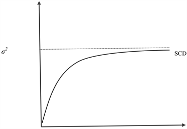
Covariance between one week returns of X_t and Y_t

$\text{Cov}\left(X_t,Y_t\right)=Cov\left(X_t,X_{t-1}\right)=0$

Because X_t series is iid.

Therefore, if we look at univariate tests for random walk behavior in asset Y, we probably will find no rejection because the return series is iid. The univariate tests of the random walk hypothesis are not powerful enough to detect this sort of a deviation from joint market efficiency. Our point is that we need to make use of the information in the off-diagonal elements of the variance-covariance matrix to test for joint market efficiency.

If k-week SCD is significant, it means that scaled k-week covariance is significantly different from scaled 1-week covariance. This suggests that there is a lag in information/shock transmission between the markets under consideration. SCD being insignificant indicates that the k-week covariance is not statistically different from 1-week covariance. This means that there is no lag in information or shock transmission between the markets. Therefore SCD serves as an indicator to test the joint efficiency of markets.

There are other practical implications for the SCD other than test for joint efficiency. In portfolio optimization, estimation of the variance-covariance matrix is of paramount importance. Scaled cov-diff helps to identify circumstances when k-week covariance depends on k. Knowing this is important for figuring out what values to use as parameter inputs in mean variance optimization framework. If the scaled k-week covariance is significantly different from 1-week covariance, then the input for mean-variance optimization depends on the value of k. That is to say, the SCD helps to identify the circumstances when k-week covariance depends on k.

2.2. Equations & Hypotheses

We consider Equation (1) and Equation (2) from Section 2.2. We test the following hypotheses

$H_1:\rho x,y=0$ $\left(H_{1a}:\rho x,y\ne 0\right)$

$H_2:k\text{-week Scaled Covariance}\left(x,y\right)=0$ $\left(H_{2a}:k\text{-week Scaled Covariance}\left(x,y\right)\ne 0\right)$

$H_3:\mathrm{V}-Ratio=1$ $\left(H_{3a}:\text{V-Ratio}\ne 1\right)$

$H_4:SCD\left(x,y\right)=0$ $\left(H_{4a}:SCD\left(x,y\right)\ne 0\right)$

3. Empirical Analysis

3.1. Data

We make use of data of weekly closing price of S&P500 and NIFTY index and data on USD-INR from Bloomberg to compute weekly log returns using the formula:

$x_t=\ln \left(\text{Closing index level on week}t\right)-\ln \left(\text{Closing index level on week}t-1\right)$

Data from January 1996 to December 2016 is used for the analysis. There is no time-overlap between the indices considered for the study. The data is time aligned i.e. the weekly data is sorted and matched according to the date. The whole sample was further sub-divided into 2 sub-samples to examine the pre-crisis and post-crisis behavior. Sub-sample#1 consists of data of weekly log returns from January 1996 to December 2007. Sub-sample#2 consists of data of weekly log returns from January 2009 to December 2016.

It is important to discuss why weekly data is considered for the analysis. The most crucial reason for conducting this study using weekly data is to avoid biases arising from non-trading days, asynchronous prices etc. Lo and MacKinlay [2] argue that weekly sampling is the ideal compromise yielding a large number of observations while minimizing the biases inherent in daily data. This argument is supported by Ramchand and Susmel (1998) who used weekly data as opposed to monthly data for the study since it provides enough observations needed to estimate the different states of correlation without the noise of daily data.

3.2. Analysis

In order to test Hypothesis I and II (H₁:ρ_x,y = 0 & H₂ :Scaled Cov_x,y =0) we compute weekly log return of S&P500 and Nifty index using the data and generate series of k-week returns using the equation specified in Section 2.2 for sub-sample#1 and sub-sample#2. The null hypothesis for each sub-sample is based on the assumption that the two series of weekly returns are independent of each other. To test this hypothesis we make use of the bootstrapping technique to generate 1000 bootstrap samples of k-week returns of S&P500 (adjusted for ) independently of the 1000 bootstrap samples of k-week returns of the Nifty index. For each of the 1000 bootstrap samples, we then compute the k-week correlation, scaled k-week covariance. We also compute the bootstrap standard error for each k-week, t-statistic with respect to 0 and upper and lower limits of the confidence interval.

To test Hypothesis III (H₃ :V-Ratio = 0), we compute the V-Ratio of Nifty and S&P500 during sub-sample#1 and sub-sample#2. Bootstrapping technique is used in order to generate reliable standard errors. The result consists of V-Ratio, Standard error, t-stat with respect to 1 and the upper and lower limits of the confidence interval.

A different bootstrapping technique is employed to test Hypothesis IV (H₄: Scaled Cov-diff = 0). In this case, we do not generate bootstrap samples for the series by considering them independent of each other. The weekly returns of Nifty and S&P500 (adjusted for ) are taken as inputs to compute SCD. Thousand bootstrap samples are generated such that each pair of returns belong to the same calendar week. The output consists of k-week SCD, standard error, t-stat with respect to 0 and upper and lower limits of the confidence interval. Our empirical findings are summarized in the next section.

3.3. Empirical Findings

The output of the analysis is summarized in the following 10 tables. Each table contains six columns that represent the k-week, correlation/scaled covariance/V-ratio/scaled cov-diff, standard error, t-statistic with respect to 0 (t-statistic with respect to 1 for V-ratio), upper and lower limits of the confidence interval. The bootstrap procedure has been made use of in order to get reliable standard errors based on the finite sample distribution of the test statistics. Figures corresponding to each table are also given.

To test the hypothesis-H1 stated in Section 2.3, we undertake t-tests, with the size of the test being α = 5%. For the sub-sample#1 (Table 1) and sub-sample#2 (Table 2), correlation remain significantly different from 0 as k-week goes from 1 to 8. It is evident from Figure 1 that beyond k-week = 3, correlation appears more or less flat. It undergoes a slight decrease in case of sub-sample #2. Based on the t-tests, we reject the null hypothesis H1 at 95% confidence level for sub-sample#1 and sub-sample#2. Further, it can be observed that the level of correlation has increased for each k-week, subsequent to the global financial crisis (i.e. during sub-sample#2) (Figure 2).

In order to check the pattern of covariance between the k-week return series of Nifty and S&P500, we computed the scaled covariance between the k-week returns of Nifty and S&P500. Table 3 and Table 4 display the results of the analysis during sub-sample#1 and sub-sample#2 respectively. The scaled covariance remains flat after k-week = 3 prior to the global financial crisis (Figure 3 & Figure 4). The t-statistic for each scaled k-week covariance is significant. Therefore we reject H2 (Section 3.2) for sub-sample#1 and sub-sample#2 at 95% confidence level except for k-week = 7 & 8 during sub-sample #2.

Table 5 and Table 6 summarize information about k-week V-ratio of Nifty index during sub-sample#1 and sub-sample#2 respectively. During sub-sample#1 the deviation of V-ratio remain significant till k-week = 4 and becomes insignificant

Table 1. ρ:k-week Correlation between Nifty and S&P 500 during sub-sample#1.

Table 1 contains 6 columns namely, correlation between weekly log-returns NIFTY and S&P500 at level, standard errors, t-statistic with respect to zero, lower and upper limits of the confidence interval during sub-sample#1 (Jan1996-Dec 2007).

Table 2. ρ:k-week Correlation between Nifty and S&P500 during sub-sample#2.

Table 2 contains 6 columns namely, correlation between weekly log-returns NIFTY and S&P500 at level, standard errors, t-statistic with respect to zero, lower and upper limits of the confidence interval during sub-sample# 2 (Jan 2009-Dec 2016).

Table 3. k-week scaled covariance between Nifty and S&P500 sub-sample#1

Table 3 contains 6 columns namely, scaled covariance between weekly log-returns NIFTY and S&P500 at level, standard errors, t-statistic with respect to zero, lower and upper limits of the confidence interval (95%) during sub-sample#1 (Jan1996-Dec 2007).

Table 4. k-week scaled covariance between Nifty and S&P500 during sub-sample#2.

Table 4 contains 6 columns namely, scaled covariance between weekly log-returns NIFTY and S&P500 at level, standard errors, t-statistic with respect to zero, lower and upper limits of the confidence interval (95%) during sub-sample#1 (Jan2009-Dec 2016).

Table 5. k-week V-Ratio of Nifty during sub-sample#1.

Table 5 contains 6 columns namely, Variance ratio of the NIFTY index, standard errors, t-statistic with respect to zero, lower and upper limits of the of confidence interval (95%) during sub-sample#1 (Jan1996-Dec 2007).

Table 6. k-week V-Ratio of Nifty during sub-sample#2.

Table 6 contains 6 columns namely, Variance ratio of the NIFTY index, standard errors, t-statistic with respect to zero, lower and upper limits of the of confidence interval (95%) during sub-sample#1 (Jan1996-Dec 2007).

Figure 1. k-week correlation (S&P500-Nifty) during sub-sample#1. Figure 1 and Figure 2 show correlation between weekly log-returns NIFTY and S&P500 at level during sub-sample#1 (Jan 1996-Dec 2007) and sub-sample#2 (Jan 2009-Dec 2016) respectively. The dashed lines form the boundaries of 95% confidence interval.

Figure 2. k-week correlation (S&P500-Nifty) during sub-sample#2. Figure 1 and Figure 2 show correlation between weekly log-returns NIFTY and S&P500 at level during sub-sample#1 (Jan 1996-Dec 2007) and sub-sample#2 (Jan 2009-Dec 2016) respectively. The dashed lines form the boundaries of 95% confidence interval.

Figure 3. k-week Scaled Covariance (S&P500-Nifty) during sub-sample#1. Figure 3 and Figure 4 show k-week scaled covariance between weekly log-returns NIFTY and S&P500 at level during sub-sample#1 (Jan 1996-Dec 2007) and sub-sample#2 (Jan 2009-Dec 2016) respectively. The dashed lines form the boundaries of 95% confidence interval.

Figure 4. k-week scaled covariance (S&P500-Nifty) during sub-sample#2. Figure 3 and Figure 4 show k-week scaled covariance between weekly log-returns NIFTY and S&P500 at level during sub-sample#1 (Jan 1996-Dec 2007) and sub-sample#2 (Jan 2009-Dec 2016) respectively. The dashed lines form the boundaries of 95% confidence interval.

Figure 5. V-Ratio of Nifty during sub-sample#1. Figure 5 and Figure 6 show V-ratio of weekly returns of Nifty index during sub-sample#1 (Jan 1996-Dec 2007) and sub-sample #2 respectively. The dotted lines form the boundaries of the 95% confidence interval.

Figure 6. V-Ratio of Nifty during sub-sample#2. Figure 5 and Figure 6 show V-ratio of weekly returns of Nifty index during sub-sample#1 (Jan 1996-Dec 2007) and sub-sample #2 respectively. The dotted lines form the boundaries of the 95% confidence interval.

afterwards. V-ratio for each k-week is insignificant during sub-sample#2. This can also be observed from Figure 5 and Figure 6. This suggests that we fail to reject the null hypothesis H3 (Section 3.2) for every k-week during sub-sample#2. But in case of sub-sample#1, V-ratio is insignificant only for longer term returns (starting from k-week = 4). Therefore we reject the H3 for k-week V-ratio for k ranging from 2 to 4.

The scaled k-week V-ratio of S&P500 index during sub-sample#1 and sub-sample#2 is summarized in Table 7 and Table 8 respectively (Also refer Figure 7 and Figure 8). During sub-sample#1 k-week V-ratio is insignificant for each k-week except for 2-week return series. The V-Ratio is clearly insignificant for each k-week returns in sub-sample#2 thereby providing strong evidence for the random walk hypothesis. (H3) is not rejected in case of S&P500 during sub-sample#1 as well as sub-sample#2 except for 2-week returns during sub-sample#1.

Table 7. k-week V-Ratio of S&P500 during sub-sample#1.

Table 7 contains 6 columns namely, Variance ratio of the S&P500 index, standard errors, t-statistic with respect to zero, lower and upper limits of the of confidence interval (95%) during sub-sample#1 (Jan 1996-Dec 2007).

Table 8. k-week V-Ratio of S&P500 during sub-sample#2.

Table 8 contains 6 columns namely, Variance ratio of the S&P500 index, standard errors, t-statistic with respect to zero, lower and upper limits of the of confidence interval (95%) during sub-sample#2 (Jan 2009-Dec 2016).

Table 9. Scaled cov-diff: Difference of k-week and 1-week Covariance (Nifty and S&P 500) during sub-sample#1.

Table 9 contains 6 columns namely, difference between k-week scaled covariance and 1-week covariance of S&P500 and NIFTY, standard errors, t-statistic with respect to zero and lower and upper limits of the 95% confidence interval during sub-sample#1.

Table 10. Scaled cov-diff: Difference of k-week and 1-week Covariance (Nifty and S&P 500) during sub-sample#2.

Table 10 contains 6 columns namely, difference between k-week scaled covariance and 1-week covariance of S&P500 and NIFTY, standard errors, t-statistic with respect to zero and lower and upper limits of the 95% confidence interval during sub-sample#2.

Figure 7. V-Ratio of S&P500 during sub-sample#1. Figure 7 and Figure 8 show V-ratio of weekly returns of S&P500 index during sub-sample#1 (Jan 1996-Dec 2007) and sub-sample#2 respectively. The dotted lines form the boundaries of the 95% confidence interval.

Figure 8. V-Ratio of S&P500 during sub-sample#2. Figure 7 and Figure 8 show V-ratio of weekly returns of S&P500 index during sub-sample#1 (Jan 1996-Dec 2007) and sub-sample#2 respectively. The dotted lines form the boundaries of the 95% confidence interval.

Figure 9. SCD (S&P500-Nifty) during sub-sample#1. Figure 9 and Figure 10 show the difference of k-week and 1-week covariance between weekly log-returns of NIFTY and S&P500 during sub-sample#1 (Jan 1996-Dec 2007) and sub-sample#2 (Jan 2009-Dec 2016) respectively. The dashed lines form the boundaries of 95% confidence interval.

Figure 10. SCD (S&P500-Nifty) during sub-sample#2. Figure 9 and Figure 10 show the difference of k-week and 1-week covariance between weekly log-returns of NIFTY and S&P500 during sub-sample#1 (Jan 1996-Dec 2007) and sub-sample#2 (Jan 2009-Dec 2016) respectively. The dashed lines form the boundaries of 95% confidence interval.

Table 9 and Table 10 show information pertaining to scaled cov-diff. Figure 9 and Figure 10 represents the information summarized in Table 9 & Table 10. Scaled cov-diff captures the difference between k-week covariance and 1-week covariance. If the value of scaled cov-diff is not statistically different from 0, it suggests that there is no lag in information transmission between the markets. In this case, US is the bigger market and Indian stock market is more like a satellite to it. Failing to reject the null-H4 (Section 3.2) indicate that the transmission of information from the US market to the Indian market happens within the same week.

We observe that the scaled cov-diff is not statistically different from 0 for k-week as k goes from 2 to 8 during sub-sample#1 and sub-sample#2 (Table 9 & Table 10). Therefore we fail to reject the null hypothesis-H4. Scaled cov-diff = 0 does not mean the scaled covariance is zero. It indicates that the scaled covariance, remains flat. It means that the markets are efficient as the information transmission happens within the same week. This is an evidence for the joint efficiency of the Indian and American stock markets.

4. Conclusion

In this study, we have introduced a new measure called the Scaled Covariance Difference (SCD), which captures the difference between the covariance of short term returns and longer-term returns. We have made use of information in the off-diagonal terms of the variance-covariance matrix in the analysis so as to develop a test for joint market efficiency. We have demonstrated how to implement the test for joint market efficiency using data on weekly stock returns from the Nifty and S&P 500 indices. What we find is that, the k-week SCD between the US and the Indian market remains insignificant for all values of k. This suggests that the information transmission between these markets occurs within the same week. This provides strong evidence for the joint efficiency of Indian and American stock markets.

Conflicts of Interest

The authors declare no conflicts of interest regarding the publication of this paper.

References

[1]	Bachelier, L. (1900) Théorie de la spéculation. Annales scientifiques de l’école Normale Supérieure, 17, 21-86. https://doi.org/10.24033/asens.476
[2]	Lo, A.W. and MacKinlay, A.C. (1988) Stock Market Prices Do Not Follow Random Walks: Evidence from a Simple Specification Test. Review of Financial Studies, 1, 41-66. https://doi.org/10.1093/rfs/1.1.41
[3]	Huang, B.N. (1995) Do Asian Stock Market Prices Follow Random Walks? Evidence from the Variance Ratio Test. Applied Financial Economics, 5, 251-256. https://doi.org/10.1080/758536875
[4]	Urrutia, J.L. (1995) Tests of Random Walk and Market Efficiency for Latin American Emerging Equity Markets. Journal of Financial Research, 18, 299-309. https://doi.org/10.1111/j.1475-6803.1995.tb00568.x
[5]	Smith, G. and Ryoo, H.J. (2003) Variance Ratio Tests of the Random Walk Hypothesis for European Emerging Stock Markets. The European Journal of Finance, 9, 290-300. https://doi.org/10.1080/1351847021000025777
[6]	Darrat, A.F. and Zhong, M. (2000) On Testing the Random-Walk Hypothesis: A Model-Comparison Approach. Financial Review, 35, 105-124. https://doi.org/10.1111/j.1540-6288.2000.tb01423.x
[7]	Geweke, J. and Feige, E. (1979) Some Joint Tests of the Efficiency of Markets for Forward Foreign Exchange. The Review of Economics and Statistics, 61, 334-341. https://doi.org/10.2307/1926062
[8]	Granger, C.W. (1986) Developments in the Study of Cointegrated Economic Variables. Oxford Bulletin of Economics and Statistics, 48, 213-228. https://doi.org/10.1111/j.1468-0084.1986.mp48003002.x
[9]	Chan, K., Gup, B. and Pan, M.S. (1992) Market Efficiency and Cointegration Tests for Foreign Currency Futures Markets. Journal of International Financial Markets, Institutions & Money, 2, 78-89.
[10]	Arshanapalli, B. and Doukas, J. (1993) International Stock Market Linkages: Evidence from the Pre- and Post-October 1987 Period. Journal of Banking & Finance, 17, 193-208. https://doi.org/10.1016/0378-4266(93)90088-U
[11]	DeFusco, R., Geppert, J. and Tsetsekos, G. (1993) Emerging Capital Markets: Results from Cointegration Tests. The Annual Meeting of the Financial Management Association.
[12]	Johansen, S. (1988) Statistical Analysis of Cointegration Vectors. Journal of Economic Dynamics and Control, 12, 231-254. https://doi.org/10.1016/0165-1889(88)90041-3
[13]	Johansen, S. (1991) Estimation and Hypothesis Testing of Cointegration Vectors in Gaussian Vector Autoregressive Models. Econometrica, 59, 1551-1580. https://doi.org/10.2307/2938278
[14]	Forbes, F.H. and Rigbon, R. (2002) No Contagion, Only Interdependence: Measuring Stock Market Comovements. The Journal of Finance, 57, 2223-2261. https://doi.org/10.1111/0022-1082.00494
[15]	Erb, C.B., Harvey, C.R. and Viskanta, T.E. (1994) Forecasting International Equity Correlations. Financial Analysts Journal, 50, 32-45. https://doi.org/10.2469/faj.v50.n6.32
[16]	Kaplanis, E.C. (1988) Stability and Forecasting of the Comovement Measures of International Stock Market Returns. Journal of International Money and Finance, 7, 63-75. https://doi.org/10.1016/0261-5606(88)90006-X
[17]	King, M.A. and Wadhwani, S. (1990) Transmission of Volatility between Stock Markets. The Review of Financial Studies, 3, 5-33. https://doi.org/10.1093/rfs/3.1.5
[18]	Koch, P.D. and Koch, T.W. (1991) Evolution in Dynamic Linkages across Daily National Stock Indexes. Journal of International Money and Finance, 10, 231-251. https://doi.org/10.1016/0261-5606(91)90037-K
[19]	Longin, F. and Solnik, B. (1995) Is the Correlation in International Equity Returns Constant: 1960-1990? Journal of International Money and Finance, 14, 3-26. https://doi.org/10.1016/0261-5606(94)00001-H
[20]	Karolyi, G.A. and Stulz, R.M. (1996) Why Do Markets Move Together? An Investigation of US-Japan Stock Return Comovements. The Journal of Finance, 51, 951-986. https://doi.org/10.1111/j.1540-6261.1996.tb02713.x
[21]	Longin, F. and Solnik, B. (2001) Extreme Correlation of International Equity Markets. The Journal of Finance, 56, 649-676. https://doi.org/10.1111/0022-1082.00340
[22]	Agarwal, A., Wong, W. and Du, J. (2005) Financial Integration for India Stock Market, a Fractional Cointegration Approach. National University of Singapore, Department of Economics, Departmental Working Papers No. wp0501. http://www.fas.nus.edu.sg/ecs/pub/wp/wp0501.pdf