The Effectiveness of the Squared Error and Higgins-Tsokos Loss Functions on the Bayesian Reliability Analysis of Software Failure Times under the Power Law Process

Freeh N. Alenezi^1,2, Christ P. Tsokos¹

¹University of South Florida, Tampa, FL, USA.
²Majmaah University, Al-Zulfi, Saudi Arabia.

DOI: 10.4236/eng.2019.115020                

Abstract

Reliability analysis is the key to evaluate software’s quality. Since the early 1970s, the Power Law Process, among others, has been used to assess the rate of change of software reliability as time-varying function by using its intensity function. The Bayesian analysis applicability to the Power Law Process is justified using real software failure times. The choice of a loss function is an important entity of the Bayesian settings. The analytical estimate of likelihood-based Bayesian reliability estimates of the Power Law Process under the squared error and Higgins-Tsokos loss functions were obtained for different prior knowledge of its key parameter. As a result of a simulation analysis and using real data, the Bayesian reliability estimate under the Higgins-Tsokos loss function not only is robust as the Bayesian reliability estimate under the squared error loss function but also performed better, where both are superior to the maximum likelihood reliability estimate. A sensitivity analysis resulted in the Bayesian estimate of the reliability function being sensitive to the prior, whether parametric or non-parametric, and to the loss function. An interactive user interface application was additionally developed using Wolfram language to compute and visualize the Bayesian and maximum likelihood estimates of the intensity and reliability functions of the Power Law Process for a given data.

Keywords

Power Law Process, Bayesian Reliability, Intensity Function, Kernel Density, Loss Function, Robustness

1. Introduction

Reliability analysis of a software under development is a key to assess whether a desired level of a quality product is achieved. Specially, when a software package is considered, and is tested after each failure detection, and then corrected until a new failure is observed. Over the past few decades, the reliability analysis of a software package has been studied, where graphical and numerical metrics have been introduced. One of the earliest, Duane (1964) [1] , who introduced a graph to assess the reliability of a software over time using its failure times. It has the cumulative failure rate and the time on the y-axis and x-axis, respectively. In this graph, one can conclude a software reliability improvement if a negative curve is observed whereas a positive curve means the software reliability is deteriorating. On the other hand, a horizontal line indicates that the software reliability is stable. The failure numbers $N\left(t\right)$ in time interval $\left(\mathrm{0,}t\right]$ is considered a Poisson counting process after satisfying the following conditions:

1) $N\left(t=0\right)=0$.

2) Independent increment (counts of disjoint time intervals are independent).

3) It has an intensity function

$V\left(t\right)=\underset{\Delta t\to 0}{\lim }\frac{P\left(N\left(t,t+\Delta t\right)=1\right)}{\Delta t}.$

4) Simultaneous failures do not exist

$\underset{\Delta t\to 0}{\lim }\frac{P\left(N\left(t,t+\Delta t\right)=2\right)}{\Delta t}=0.$

The probability of random value $N\left(t\right)=n$ is given by:

$P\left(N\left(t\right)=n\right)=\frac{\exp \left\{-{\displaystyle {\int }_0^t}V\left(t\right)\text{d}t\right\}{\left\{{\displaystyle {\int }_0^t}V\left(t\right)\text{d}t\right\}}^n}{n!},t>0.$ (1)

Crow (1974) proposed a Non-Homogeneous Poisson Process (NHPP) , which is a Poisson Process with a time varying intensity function, given by:

$V\left(t\right)=V\left(t;\beta ,\theta \right)=\frac{\beta }{\theta }{\left(\frac{t}{\theta }\right)}^{\beta -1},t>0,\beta >0,\theta >0,$ (2)

with $\beta$ and $\theta$ are the shape and scale parameters, respectively. This Non-Homogeneous Poisson Process is also known as the Power Law Process (PLP).

The joint probability density function (PDF) of the ordered failure times $T_1,T_2,\cdots ,T_n$ from a NHPP with intensity function $V\left(t\mathrm{<mo>\; ;\; </mo>}\beta \mathrm{,}\theta \right)$ is given by:

$f\left(t_1,\cdots ,t_n\right)={\displaystyle {\prod }_{i=1}^{n}V\left(t_i;\beta ,\theta \right)\exp \left\{-{\displaystyle {\int }_0^w}V\left(t;\beta ,\theta \right)\text{d}t\right\}},$ (3)

where w is the so-called stopping time; $w=t_n$ for the failure truncated case. Considering the failure truncation case, the conditional reliability function of the failure time $T_n$ given $T_1=t_1$, $T_2=t_2$, $T_3=t_3$, $\cdots$, $T_{n-2}=t_{n-2}$, $T_{n-1}=t_{n-1}$ is a function of $V\left(t\mathrm{<mo>\; ;\; </mo>}\beta \mathrm{,}\theta \right)$.

As a numerical assessment, the estimate of the key parameter $\beta$ in the $V\left(t\mathrm{<mo>\; ;\; </mo>}\beta \mathrm{,}\theta \right)$ has an important role in evaluating the reliability of a software package. When the estimates of $\beta$ are less and larger than 1, they indicate that the software reliability is improving and decreasing, respectively. The PLP is reduced to a homogeneous Poisson process when the estimate of $\beta$ equals to 1.

The NHPP has been used for analyzing software’s failure times, and prediction of the next failure time. The subject model has been shown to be effective and useful not only in software reliability assessment [2] - [11] , but also in cyber-security; the attack detection in cloud systems [12] [13] , breast and skin cancer treatments’ effectiveness, [14] [15] [16] , respectively, finance; modeling of financial markets at the ultra-high frequency level [17] , trnasportation; modeling passengers’ arrivals [18] [19] [20] [21] [22] , and in the formulation of a software cost model [23] .

Since the conditional reliability function of the PLP is a function of the $V\left(t\mathrm{<mo>\; ;\; </mo>}\beta \mathrm{,}\theta \right)$, which includes the key parameter $\beta$. That being said updating the estimation methods for the key parameter will affect positively the $V\left(t\mathrm{<mo>\; ;\; </mo>}\beta \mathrm{,}\theta \right)$ and the software reliability estimation, and therefore help the structuring of maintenance strategies. The authors [24] and [25] obtained the Bayesian estimates of the parameter $\beta$ under the the squared-error and Higgins-Tsokos loss functions, respectively, and compared them to their approximate maximum likelihood estimate (MLE). They also showed the superiority of the Bayesian estimates to the MLE of the key parameter $\beta$, and the improvement in the reliability assessment under the PLP.

To perform Bayesian analysis on a real world problem, one needs to justify the applicability of such analysis. Then, the analysis process starts by identifying the probability distribution of the failure times of a software under development, the prior PDF of the key parameter $\beta$, and a loss function. The analytical tractability have made the squared-error loss function commonly used, where it places more weight on the estimates that are far from the true value than the estimates close to true value. Higgins and Tsokos [26] proposed a new loss function that maintains the analytical tractability feature and places exponentially more weight on extreme estimates of the true value.

In the present study, we investigate the effectiveness, in Bayesian Analysis, of using the commonly used squared-error (S-E) loss function versus the Higgins-Tsokos (H-T) loss function that puts the loss at the end of the process, for modeling software failure times. To accomplish this, we used the underline failure distribution to be the Power Law Process subject to using Burr PDF as a prior of the key parameter $\beta$. In addition, we utilize both loss functions to perform sensitive analysis of the prior selections. We perform parametric and non-parametric priors, namely Burr, Inverted Gamma, Jeffery, and two Kernel PDFs. Therefore, the primary objective of the study is to answer the following questions within a Bayesian framework:

1) How robust is the assumption of the squared-error loss function being challenged by the Higgins-Tsokos loss function in estimating the key parameter $\beta$ of PLP for modeling software failure times?

2) Is the Bayesian estimate of the intensity function, $V\left(t\mathrm{<mo>\; ;\; </mo>}\beta \mathrm{,}\theta \right)$, of the PLP sensitive to the selections of the prior (parametric and non-parametric) and loss function (Higgins-Tsokos and S-E loss functions)?

The paper is organized as follows, Section 2 describes the theory and development of the Bayesian reliability model. Section 3 presents the results and discussion. Section 4 are the conclusions.

2. Theory and Bayesian Estimates

2.1. Review of the Analytical Power Law Process

The probability of achieving n failures of a given system in the time interval

$\left(\mathrm{0,}t\right]$ can be written as

$P\left(x=n;t\right)=\frac{\exp \left\{-{\displaystyle {\int }_0^t}V\left(x\right)\text{d}x\right\}{\left\{{\displaystyle {\int }_0^t}V\left(x\right)\text{d}x\right\}}^n}{n!},t>0,$ (4)

where $V\left(t\right)$ is the intensity function given by (2). The reduced expression is given by:

$P\left(x=n;t\right)=\frac{1}{n!}\exp \left\{-{\frac{t}{\theta }}^{\beta }\right\}{\frac{t}{\theta }}^{n\beta },$ (5)

is the PLP that is commonly known as Weibull or Non-Homogeneous Poisson Process.

When the PLP is the underlying failure model of the failure times $t_1,t_2,t_3,\cdots ,t_{n-1}$ and $t_n$, the conditional reliability function of $t_n$ given $t_1,t_2,t_3,\cdots ,t_{n-1}$ can be written mathematically as a function of the intensity function, given by:

$R\left(t_n|t_1,t_2,\cdots ,t_{n-1}\right)=\exp \left\{{\displaystyle {\int }_{t_{n-1}}^{t_n}}-V\left(t;\beta ,\theta \right)\text{d}t\right\},t_n>t_{n-1}>0,$ (6)

since it is independent of $t_1,t_2,t_3,\cdots ,t_{n-2}$.

Note that the improvement in estimating the key parameter $\beta$ in the $R\left(t_n\mathrm{<mo>\; |\; </mo>}{t}_1\mathrm{,}{t}_2\mathrm{,}\cdots \mathrm{,}{t}_{n-1}\right)$ of the PLP, Equation (6), will improve the reliability estimation.

The maximum likelihood estimation (MLE) of $\beta$ is a function of the largest failure time and the MLE of $\theta$ is also a function of the MLE of $\beta$. Let

$T_1,T_2,\cdots ,T_n$ denote the first n failure times of the PLP, where $T_l<T_2<\cdots <T_n$

are measured in global time; that is, the times are recorded since the initial startup of the system. Thus, the truncated conditional probability distribution function, $f_i\left(t\mathrm{<mo>\; |\; </mo>}{t}_1\mathrm{,}\cdots \mathrm{,}{t}_{i-1}\right)$, in the Weibull process is given by

$f_i\left(t|t_1,\cdots ,t_{i-1}\right)=\frac{\beta }{\theta }{\left(\frac{t}{\theta }\right)}^{\beta -1}\exp \left\{-{\frac{t}{\theta }}^{\beta }+{\frac{t_{i-1}}{\theta }}^{\beta }\right\},t_{i-1}<t.$ (7)

With $t=\left(t_1,t_2,.\cdots ,t_n\right)$, the Likelihood function for the first n failure times of the PLP $T_1=t_1,T_2=t_2,\cdots ,T_n=t_n$ can be written as

$L\left(t,\beta \right)=\exp \left(-{\left(\frac{t_n}{\theta }\right)}^{\beta }\right){\left(\frac{\beta }{\theta }\right)}^n{\displaystyle \underset{i=1}{\overset{n}{\prod }}}{\left(\frac{t_i}{\theta }\right)}^{\beta -1}.$ (8)

The MLE for the shape parameter is given by

${\hat{\beta }}_n=\frac{n}{{\displaystyle {\sum }_{i=1}^n\log \left(\frac{t_n}{t_i}\right)}},$ (9)

and for the scale parameter is

${\hat{\theta }}_n=\frac{t_n}{n^{1/{\hat{\beta }}_n}}.$ (10)

Note that the MLE of $\theta$ depends on the MLE of $\beta$.

2.2. Development of the Bayesian Estimates

The authors [24] and [25] justified the applicability of Bayesian analysis to the PLP based on the Crow, [2] [27] , failure data from a system undergoing developmental testing (Table 1), by showing that the MLE of the key parameter $\beta$ varies depending on the last failure time (largest time). Moreover, the authors used the Crow data (40 successive failure times) to compute the MLE of $\beta$ ( ${\hat{\beta }}_{40}=0.49$ ), then computed the estimate considering the $t_{39}=3181$ is the largest failure time ( ${\hat{\beta }}_{39}=0.48$ ) and so on. After computing all MLEs of the key parameter $\beta$, they found that the MLEs of $\beta$ follows a four-parameter Burr probability distribution, $g\left(\beta \mathrm{<mo>\; ;\; </mo>}\alpha \mathrm{,}\gamma \mathrm{,}\delta \mathrm{,}\kappa \right)$, known as the four-parameter Burr type XII probability distribution, with a PDF given by:

$g_B\left(\beta \right)=g\left(\beta ;\alpha ,\gamma ,\delta ,\kappa \right)=\{\begin{array}{l}\frac{\alpha \kappa {\left(\frac{\beta -\gamma }{\delta }\right)}^{\alpha -1}}{\delta {\left(1+{\left(\frac{\beta -\gamma }{\delta }\right)}^{\alpha }\right)}^{\kappa +1}}\gamma \le \beta <\infty \\ 0\text{otherwise}\end{array}$ (11)

where the hyperparameters $\alpha$, $\gamma$, $\delta$ and $\kappa$ are being estimated using MLEs in the Goodness of Fit (GOF) test applied to the $\beta$ estimates. The MLE

Table 1. Crow’s failure times of a system under development.

of the key parameter $\beta$ is always affected by the largest failure, and therefore it is recommended not to consider it unknown constant. This recommendation provides the opportunity to study Bayesian analysis in the PLP with respect to various selections of loss functions and priors.

The Bayesian estimates of $\beta$ will be derived using the squared-error and Higgins-Tsokos loss functions.

2.2.1. Bayesian Estimates Using Squared Error (S-E) Loss Function

The S-E loss function is given by:

$L\left(\hat{\xi },\xi \right)={\left(\hat{\xi }-\xi \right)}^2.$ (12)

The risk using the S-E loss function, where $\xi =\beta$ represents the estimate of $\hat{\xi }=\hat{\beta }$, is given by:

$E\left[L\left(\hat{\beta }\mathrm{,}\beta \right)\right]={\displaystyle {\int }_{-\infty }^{\infty }}\left[{\left(\hat{\beta }-\beta \right)}^2\right]h\left(\beta \mathrm{<mo>\; |\; </mo>}t\right)\text{d}\beta \mathrm{,}$ (13)

By differentiating $E\left[L\left(\hat{\beta }\mathrm{,}\beta \right)\right]$ with respect to $\beta$ and setting it equal to zero we solve for $\hat{\beta }$, the Bayesian estimate of $\beta$ with respect to the S-E loss function and Burr probability distribution, Equation (11), given by:

${\hat{\beta }}_{B.SE}={\displaystyle {\int }_{-\infty }^{\infty }}\beta \cdot h\left(\beta |t\right)\text{d}\beta ,$ (14)

where the posterior PDF of $\beta$ given data (t), $h\left(\beta \mathrm{<mo>\; |\; </mo>}t\right)$, using the Bayes?? theorem, is given by:

$h\left(\beta |t\right)=\frac{L\left(t|\beta \right)g_B\left(\beta \right)}{{\displaystyle {\int }_{-\infty }^{\infty }}L\left(t|\beta \right)g_B\left(\beta \right)\text{d}\beta }.$ (15)

Then, the Bayesian estimate of $\beta$, under the squared-error loss, is given by

${\hat{\beta }}_{B.SE}=\frac{{\displaystyle {\int }_{\gamma }^{\infty }}\frac{{\beta }^{n+1}}{{\theta }^n}\exp \left\{-{\left(\frac{t_n}{\theta }\right)}^{\beta }\right\}{\displaystyle {\prod }_{i=1}^n{\left(\frac{t_i}{\theta }\right)}^{\beta -1}}\frac{{\left(\frac{\beta -\gamma }{\delta }\right)}^{\alpha -1}}{{\left(1+{\left(\frac{\beta -\gamma }{\delta }\right)}^{\alpha }\right)}^{\kappa +1}}\text{d}\beta }{{\displaystyle {\int }_{\gamma }^{\infty }}\frac{{\beta }^n}{{\theta }^n}\exp \left\{-{\left(\frac{t_n}{\theta }\right)}^{\beta }\right\}{\displaystyle {\prod }_{i=1}^n{\left(\frac{t_i}{\theta }\right)}^{\beta -1}}\frac{{\left(\frac{\beta -\gamma }{\delta }\right)}^{\alpha -1}}{{\left(1+{\left(\frac{\beta -\gamma }{\delta }\right)}^{\alpha }\right)}^{\kappa +1}}\text{d}\beta }.$ (16)

2.2.2. Bayesian Estimates Using the Higgins-Tsokos Loss Function

The H-T loss function (1976) is given by

$L\left(\hat{\xi },\xi \right)=\frac{f_1\exp \left\{f_2\left(\hat{\xi }-\xi \right)\right\}+f_2\exp \left\{-f_1\left(\hat{\xi }-\xi \right)\right\}}{f_1+f_2}-1,f_1,f_2>0.$ (17)

Higgins and Tsokos [26] showed that it places more weight on the extreme underestimation and overestimation when $f_1>f_2$ and $f_1<f_2$, respectively. The risk using the H-T loss function, where $\xi =\beta$ represents the estimate of $\hat{\xi }=\hat{\beta }$, is given by:

$E\left[L\left(\hat{\beta },\beta \right)\right]={\displaystyle {\int }_{-\infty }^{\infty }}\left[\frac{f_1\exp \left\{f_2\left(\hat{\beta }-\beta \right)\right\}+f_2\exp \left\{-f_1\left(\hat{\beta }-\beta \right)\right\}}{f_1+f_2}-1\right]h\left(\beta |t\right)\text{d}\beta$ (18)

By differentiating $E\left[L\left(\hat{\beta }\mathrm{,}\beta \right)\right]$ with respect to $\beta$ and setting it equal to zero we solve for $\hat{\beta }$, the Bayesian estimate of $\beta$ with respect to the H-T loss function, given by:

${\hat{\beta }}_{B.TH}=\frac{1}{f_1+f_2}\ln \left[\frac{{\displaystyle {\int }_{-\infty }^{\infty }}\exp \left\{f_1\beta \right\}h\left(\beta |t\right)\text{d}\beta }{{\displaystyle {\int }_{-\infty }^{\infty }}\exp \left\{-f_2\beta \right\}h\left(\beta |t\right)\text{d}\beta }\right].$ (19)

The Bayesian estimate of $\beta$ with respect to the Higgins-Tsokos loss function and Burr probability distribution, as the prior, has $h\left(\beta \mathrm{<mo>\; |\; </mo>}t\right)$ given by

$h\left(\beta |t\right)=\frac{{\left(\frac{\beta }{\theta }\right)}^n\exp \left\{-{\left(\frac{t_n}{\theta }\right)}^{\beta }\right\}{\displaystyle {\prod }_{i=1}^n{\left(\frac{t_i}{\theta }\right)}^{\beta -1}}\frac{{\left(\frac{\beta -\gamma }{\delta }\right)}^{\alpha -1}}{{\left(1+{\left(\frac{\beta -\gamma }{\delta }\right)}^{\alpha }\right)}^{\kappa +1}}\text{d}\beta }{{\displaystyle {\int }_{\gamma }^{\infty }}{\left(\frac{\beta }{\theta }\right)}^n\exp \left\{-{\left(\frac{t_n}{\theta }\right)}^{\beta }\right\}{\displaystyle {\prod }_{i=1}^n{\left(\frac{t_i}{\theta }\right)}^{\beta -1}}\frac{{(\frac{\beta -\gamma }{\delta })}^{\alpha -1}}{{\left(1+{\left(\frac{\beta -\gamma }{\delta }\right)}^{\alpha }\right)}^{\kappa +1}}\text{d}\beta }.$ (20)

With the use of Equation (6), the conditional reliability of $t_i$, the analytical structure of the conditional Bayesian reliability estimate for the PLP that is subject to the above information is given by:

${\hat{R}}_B\left(t_i|t_1,t_2,\cdots ,t_{i-1}\right)=\exp \left\{-{\displaystyle {\int }_{t_{i-1}}^{t_i}}{{\hat{V}}^{\prime }}_B\left(t;\beta ,\theta \right)\text{d}t\right\},t_i>t_{i-1}>0,$ (21)

where

${{\hat{V}}^{\prime }}_B\left(t;{\hat{\beta }}_{B^{*}},\theta \right)=\frac{{\hat{\beta }}_{B^{*}}}{\theta }{\left(\frac{t}{\theta }\right)}^{{\hat{\beta }}_{B^{*}}-1},\theta >0,t>0,$ (22)

where ${\hat{\beta }}_{B^{*}}$ is the Bayesian estimate using ${\hat{\beta }}_{B\mathrm{.}SE}$ or ${\hat{\beta }}_{B\mathrm{.}TH}$ for the squared error or Higgins-Tsokos loss functions, respectively. We are also interested in comparing the Bayesian estimates, using Higgins-Tsokos loss function, of the subject parameter for different parametric and non-parametric priors, and with respect to its MLE given by Equation (9), assuming $\beta$ has a random behavior and $\theta$ as known; as well as, comparing Equation (10) with an adjusted MLE considered as a function of $\beta$.

2.3. Sensitivity Analysis: Prior and Loss Function

In this section, we seek the answer to the following question: Is the Bayesian MLE estimate of the intensity function, $V\left(t\mathrm{<mo>\; ;\; </mo>}\beta \mathrm{,}\theta \right)$, of the PLP sensitive to the selections of the prior( parametric and non-parametric) and loss function (Higgins-Tsokos and S-E loss functions)? Assuming $\beta$ is a random variable, using simulated data, sensitive analysis was done for the following parametric and non-parametric priors ( [25] ):

1) Jeffreys’ prior ( [28] ): Jeffreys’ prior is proportional to the square root of the determinant of the Fisher information matrix ( $I\left(\beta \right)$ ). It is a non-informative prior, where the Jeffreys?? prior for the key parameter of the PLP $I\left(\beta \right)$ is scalar in this case, is given by:

$g_J\left(\beta \right)\propto \sqrt{I\left(\beta \right)}=\sqrt{-E\left(\frac{{\partial }^2\log L\left(t;\beta \right)}{\partial {\beta }^2}\right)}\propto \frac{1}{\beta },\beta >0.$ (23)

2) The inverted gamma: The PLP and inverted gamma probability distributions belong to the exponential family of probability distributions, which makes the latter a logical choice for an informative parametric prior for $\beta$. The inverted gamma probability distribution is given by:

$g_{IG}\left(\beta \right)\propto {\left(\frac{\mu }{\beta }\right)}^{v+1}\frac{1}{\mu \Gamma \left(v\right)}\exp \left\{\frac{-\mu }{\beta }\right\},\beta >0,\mu >0,v>0,$ (24)

where v and $\mu$ are the shape and scale parameters.

3) Kernel’ prior:

The kernel probability density estimation is a non-parametric method to approximately estimate the PDF of $\beta$ using a finite data set. It is given by:

$g_K\left(\beta \right)=\frac{1}{nh}{\displaystyle \underset{i=1}{\overset{n}{\sum }}}K\left(\frac{\beta -{\beta }_i}{h}\right),$ (25)

where K is the kernel function and h is a positive number called the bandwidth.

2.3.1. The Jeffreys’ Prior

Assuming Jeffreys’ PDF (23) as the prior of $\beta$ and using the likelihood (8) and (15), the posterior density of $\beta$ is:

$h_J\left(\bar{t}|\beta \right)=\frac{\exp \left\{{\left(\frac{t_n}{\theta }\right)}^{\beta }\right\}\frac{{\beta }^{n-1}}{{\theta }^{n\beta }}{\displaystyle {\prod }_{i=1}^n{\left(t_i\right)}^{\beta -1}}}{{\displaystyle {\int }_0^{\infty }}\exp \left\{{\left(\frac{t_n}{\theta }\right)}^{\beta }\right\}\frac{{\beta }^{n-1}}{{\theta }^{n\beta }}{\displaystyle {\prod }_{i=1}^n{\left(t_i\right)}^{\beta -1}}\text{d}\beta }.$ (26)

Thus, the Jeffreys’ Bayesian estimate of the key parameter $\beta$ under the S-E and H-T loss functions, using (14) and (19), are given by:

${\hat{\beta }}_{B\mathrm{.}SE}^J={\displaystyle {\int }_0^{\infty }}\beta \cdot h_J\left(\bar{t}\mathrm{<mo>\; |\; </mo>}\beta \right)\text{d}\beta \mathrm{,}$ (27)

and

${\hat{\beta }}_{B.HT}^J=\frac{1}{f_1+f_2}\ln \left[\frac{{\displaystyle {\int }_0^{\infty }}\exp \left\{f_1\beta \right\}{h}_J\left(\bar{t}|\beta \right)\text{d}\beta }{{\displaystyle {\int }_0^{\infty }}\exp \left\{-f_2\beta \right\}{h}_J\left(\bar{t}|\beta \right)\text{d}\beta }\right].$ (28)

We must rely on a numerical estimation because we cannot obtain close solutions for both ${\hat{\beta }}_{B\mathrm{.}SE}^J$ and ${\hat{\beta }}_{B\mathrm{.}HT}^J$. Also note that it depends on knowing or being able to estimate the scale parameter $\theta$.

2.3.2. The Inverted Gamma Prior

The following is an examination of the problem when the prior density of $\beta$ is given by the inverted gamma (24). Using the likelihood (8), the posterior density of $\beta$ is given by:

$h_{IG}\left(t|\beta \right)=\frac{\frac{{\beta }^{n-v-1}}{{\theta }^{n\beta }}\exp \left\{-{\left(\frac{t_n}{\theta }\right)}^{\beta }-\frac{\mu }{\beta }\right\}{\displaystyle {\prod }_{i=1}^n{\left(t_i\right)}^{\beta -1}}}{{\displaystyle {\int }_0^{\infty }}\frac{{\beta }^{n-v-1}}{{\theta }^{n\beta }}\exp \left\{-{\left(\frac{t_n}{\theta }\right)}^{\beta }-\frac{\mu }{\beta }\right\}{\displaystyle {\prod }_{i=1}^n{\left(t_i\right)}^{\beta -1}}\text{d}\beta }.$ (29)

Thus, the Bayesian estimates of $\beta$ under the inverted gamma with respect to the S-E and H-T loss functions, using (14) and (19), are given by:

${\hat{\beta }}_{B\mathrm{.}SE}^{IG}={\displaystyle {\int }_0^{\infty }}\beta \cdot h_{IG}\left(\bar{t}\mathrm{<mo>\; |\; </mo>}\beta \right)\text{d}\beta \mathrm{,}$ (30)

and

${\hat{\beta }}_{B.HT}^{IG}=\frac{1}{f_1+f_2}\ln \left[\frac{{\displaystyle {\int }_0^{\infty }}\exp \left\{f_1\beta \right\}{h}_{IG}\left(t|\beta \right)\text{d}\beta }{{\displaystyle {\int }_0^{\infty }}\exp \left\{-f_2\beta \right\}{h}_{IG}\left(t|\beta \right)\text{d}\beta }\right].$ (31)

Here as well, we must rely on a numerical estimation because we cannot obtain close solutions for ${\hat{\beta }}_{B\mathrm{.}SE}^{IG}$ and ${\hat{\beta }}_{B\mathrm{.}HT}^{IG}$. Also note that it depends on knowing or being able to estimate the scale parameter $\theta$.

2.3.3. The Kernel Prior

Assuming Kernel density (25) as the prior of $\beta$ and using the likelihood (8), the posterior density of $\beta$ is:

$h_k\left(\bar{t}|\beta \right)=\frac{\exp \left\{{\left(\frac{t_n}{\theta }\right)}^{\beta }\right\}\frac{{\beta }^n}{{\theta }^{n\beta }}{\displaystyle {\prod }_{i=1}^n{\left(t_i\right)}^{\beta -1}}\frac{1}{nh}{\displaystyle {\sum }_{i=1}^{n}K\left(\frac{\beta -{\beta }_i}{h}\right)}}{{\displaystyle {\int }_0^{\infty }}\exp \left\{{\left(\frac{t_n}{\theta }\right)}^{\beta }\right\}\frac{{\beta }^n}{{\theta }^{n\beta }}{\displaystyle {\prod }_{i=1}^n{\left(t_i\right)}^{\beta -1}}\frac{1}{nh}{\displaystyle {\sum }_{i=1}^{n}K\left(\frac{\beta -{\beta }_i}{h}\right)}\text{d}\beta }.$ (32)

Thus, the kernel Bayesian estimates of the key parameter $\beta$ under the S-E and H-T loss functions, (14) and (19), are given by:

${\hat{\beta }}_{B.SE}^K={\displaystyle {\int }_0^{\infty }}\beta \cdot h_K\left(\bar{t}|\beta \right)\text{d}\beta ,$ (33)

and

${\hat{\beta }}_{B.HT}^K=\frac{1}{f_1+f_2}\ln \left[\frac{{\displaystyle {\int }_{\gamma }^{\infty }}\exp \left\{f_1\beta \right\}{h}_k\left(\bar{t}|\beta \right)\text{d}\beta }{{\displaystyle {\int }_{\gamma }^{\infty }}\exp \left\{-f_2\beta \right\}{h}_k\left(\bar{t}|\beta \right)\text{d}\beta }\right].$ (34)

We must rely on a numerical estimation because we cannot obtain close solutions for ${\hat{\beta }}_{B\mathrm{.}SE}^K$ and ${\hat{\beta }}_{B\mathrm{.}HT}^K$. Also note that it depends on knowing or being able to estimate the scale parameter $\theta$. In addition, the kernel function, $K\left(u\right)$, and bandwidth, h, will be chosen to minimize the asymptotic mean integrated squared error (AMISE) given by:

$\text{AMISE}\left(\hat{f}\left(\beta \right)\right)={\displaystyle \int }E\left[{\left(\hat{f}\left(\beta \right)-f\left(\beta \right)\right)}^2\right]\text{d}\beta \mathrm{,}$ (35)

where $\hat{f}\left(\beta \right)$ and $f\left(\beta \right)$ are the estimated probability density of $\beta$ and the true probability density of $\beta$ respectively.

Table 2 shows the acronyms and notations used in this study.

3. Results and Discussion

3.1. Numerical Simulation

A Monte Carlo simulation was used to compare the Bayesian, under the S-E and H-T loss functions, and the MLE approaches. The parameter $\beta$ of the intensity function for the PLP was calculated using numerical integration techniques in conjunction with a Monte Carlo simulation to obtain its Bayesian estimates. Substituting these estimates in the intensity function we obtained the Bayesian intensity function estimates, from which the reliability function can be estimated.

For a given value of the parameter $\theta$, a stochastic value for the parameter $\beta$ was generated from a prior probability density. For a pair of values of $\theta$ and $\beta$, 400 samples of 40 failure times that follow a PLP were generated. This procedure was repeated 250 times and for three distinct values of $\theta$. The procedure is based on the schematic diagram given by Algorithm 1.

Table 2. Acronyms and notations used in this study.

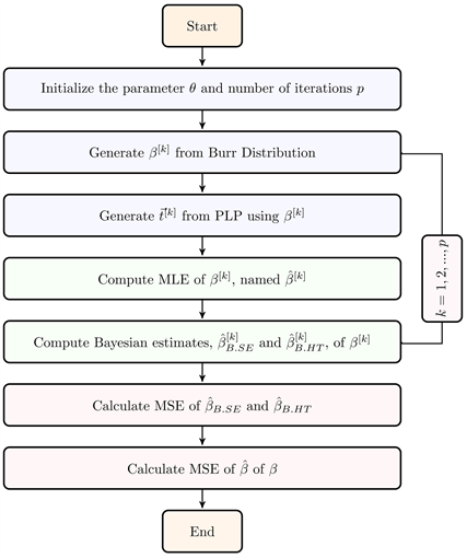
Algorithm 1. Simulation to analyze Bayesian estimates of $\beta$ for a given $\theta$.

For each sample of size 40, the Bayesian estimates and MLEs of the parameter were calculated when $\theta \in \left\{0.5,1.7441,4\right\}$. The comparison is based on the mean squared error (MSE) averaged over the 100000 repetitions. The results are given in Table 3. It is observed that ${\hat{\beta }}_{B\mathrm{.}SE}$ and ${\hat{\beta }}_{B\mathrm{.}HT}$ maintain similar accuracy, where both are superior to $\hat{\beta }$ in estimating $\beta$.

For different sample sizes, the Bayesian estimates under S-E and H-T loss functions and the MLEs of the parameter $\beta$ were calculated and averaged over 10,000 repetitions. Table 4 displays the simulated result of comparing a true value of $\beta$ with respect to its MLE and Bayesian estimates for $n=20,30,\cdots ,160$.

It can be observed that the Bayesian estimates of $\beta$ are closer to the true value than the MLE of $\beta$, where the Bayesian estimate under the H-T loss function is slightly performing better even for a very small sample size of $n=20$. A graphical comparison of the true estimate of $\beta$ along with the Bayesian estimates (under both S-E and H-T loss functions) and MLE as a function of sample size is given in Figure 1.

Figure 1 shows the the excellent performance of he Bayesian estimates compared to the MLE of the key parameter $\beta$. The Bayesian estimates tend to underestimate while while the MLE estimate tends to overestimate the true value, especially for small sample sizes. The MSEs of the MLE and Bayesian estimates of $\beta$ for each sample size are given below by Figure 2.

Figure 1. $\beta$ estimates versus sample size.

Figure 2. MSE of $\beta$ Bayesian estimates versus sample size.

Table 3. MSE for Bayesian estimates, under squared error and Higgin-Tsokos loss functions, and MLEs of $\beta$.

For the considered sample sizes, the MSEs of the Bayesian estimates of $\beta$ are sufficiently smaller than the MSEs for the MLE of $\beta$. The Bayesian estimate under the H-T loss function performed slightly better than the Bayesian estimate under the S-E loss function.

Table 4. Bayesian estimates, under squared error and Higgin-Tsokos loss functions, and MLEs for the parameter $\beta =0.7054$ averaged over 10,000 repetitions.

Since the Bayesian estimates under both loss functions for $\beta$ are superior to its MLE, Molinares and Tsokos [24] showed the improvement in the scale paramter ( $\theta$ ) when its estimate (10) is adjusted by using the Bayesian estimate of $\beta$ instead of the corresponding MLE. Therefore, we calculated the adjusted estimate of $\theta$ using MLE and Bayesian estimates under S-E and H-T loss functions of $\beta$, shown in Table 5.

This proposed adjusted estimates, ${\hat{\theta }}_{B\mathrm{.}SE}$ and ${\hat{\theta }}_{B\mathrm{.}HT}$, were averaged over the 10,000 repetitions. It can be appreciated that, based on the Bayesian influence on $\beta$, ${\hat{\theta }}_{B\mathrm{.}SE}$ and ${\hat{\theta }}_{B\mathrm{.}HT}$ are better estimates than the MLE of $\theta$ ( $\hat{\theta }$ ). This also can be seen in Figure 3, which visualize the performance of ${\hat{\theta }}_{B\mathrm{.}SE}$ and ${\hat{\theta }}_{B\mathrm{.}HT}$ compared to the corresponding MLE.

Figure 3 shows the excellent performance of the adjusted estimates of $\theta$, where the adjusted estimate under the H-Twas slightly closer to the true value. The MSEs of these estimates of $\theta$ are displayed in Figure 4 given below.

The MSEs of the adjusted estimates of the shape parameter ( $\theta$ ) are significantly smaller that the MSEs of the MLE estimate. The MSEs of the adjusted estimates are then displayed alone in Figure 5 to look closer at their performance.

It can be noticed that the adjusted estimate of $\theta$ under the influence of the Bayesian estimate with the H-T loss function, is better, particularly when considering small sample sizes.

We computed the adjusted estimate for the parameter $\theta$ and its MSE over 10000 repetitions for different values of $\theta$ and sample size $n=40$. The results are given in Table 6.

The adjusted estimate of $\theta$ are were more accurate when considering small true values of $\theta$ than the larger values.

Figure 3. $\theta$ estimates versus sample size.

Figure 4. MSE of $\theta$ Bayesian and MLE estimates versus sample size.

Figure 5. MSE of $\theta$ Bayesian estimates versus sample size.

Table 5. MLE Bayesian estimates, under squared error and Higgin-Tsokos loss functions, and and MLEs for the parameter $\theta =1.7441$ averaged over 10,000 repetitions.

Table 6. MSE of $\theta$ estimates using Bayesian estimates, under squared error and Higgin-Tsokos loss functions, and MLE of $\beta$.

The slight improvements in the estimation of the shape and scale parameters of the PLP is expected to jointly improve the estimate of the intensity function and therefore the reliability estimation of a software. For a fixed value of $\theta =1.7441$ and a sample size similar to the size of the collected data, $n=40$, the estimates of the intensity function ${\hat{V}}_{MLE}\left(t\right)$, ${\hat{V}}_{B\mathrm{.}SE}\left(t\right)$, and ${\hat{V}}_{B\mathrm{.}HT}\left(t\right)$ were obtained when we use $\hat{\beta }$, ${\hat{\beta }}_{B\mathrm{.}SE}$, and ${\hat{\beta }}_{B\mathrm{.}HT}$, respectively, in (2). That is,

${{\hat{V}}^{\prime }}_{MLE}\left(t\right)=\frac{\hat{\beta }}{\theta }{\left(\frac{t}{\theta }\right)}^{\hat{\beta }-1},\theta >0,t>0.$ (36)

${{\hat{V}}^{\prime }}_{B.SE}\left(t\right)=\frac{{\hat{\beta }}_{B.SE}}{\theta }{\left(\frac{t}{\theta }\right)}^{{\hat{\beta }}_{B.SE}-1},\theta >0,t>0.$ (37)

${{\hat{V}}^{\prime }}_{B.HT}\left(t\right)=\frac{{\hat{\beta }}_{B.HT}}{\theta }{\left(\frac{t}{\theta }\right)}^{{\hat{\beta }}_{B.HT}-1},\theta >0,t>0.$ (38)

Their graphs (Figure 6) reveal the superior performance of ${{\hat{V}}^{\prime }}_{B\mathrm{.}SE}\left(t\right)$ and ${{\hat{V}}^{\prime }}_{B\mathrm{.}HT}\left(t\right)$.

In order to obtain Bayesian estimates of the intensity function, ${\hat{V}}_{B\mathrm{.}SE}^{\ast }$ and ${\hat{V}}_{B\mathrm{.}HT}^{\ast }$, we substituted the Bayesian estimates of $\beta$ and its corresponding $\theta$ MLE in (2):

Figure 6. Graph for $\theta =1.7441$ and the corresponding $\beta$ Bayesian estimates and MLE’s used in ${{\hat{V}}^{\prime }}_{MLE}$, ${{\hat{V}}^{\prime }}_{B\mathrm{.}SE}$, and ${{\hat{V}}^{\prime }}_{B\mathrm{.}HT}$ (of time t) , n = 40.

${\hat{V}}_{B.SE}^{\ast }\left(t\right)=\frac{{\hat{\beta }}_{B.SE}}{\hat{\theta }}{\left(\frac{t}{\hat{\theta }}\right)}^{{\hat{\beta }}_{B.SE}-1},t>0.$ (39)

${\hat{V}}_{B.HT}^{\ast }\left(t\right)=\frac{{\hat{\beta }}_{B.HT}}{\hat{\theta }}{\left(\frac{t}{\hat{\theta }}\right)}^{{\hat{\beta }}_{B.HT}-1},t>0.$ (40)

The MLE of the intensity function, ${\hat{V}}_{MLE}$, is obtained using the MLEs of $\beta$ and $\theta$. That is,

${\hat{V}}_{MLE}\left(t\right)=\frac{\hat{\beta }}{\hat{\theta }}{\left(\frac{t}{\hat{\theta }}\right)}^{\hat{\beta }-1},t>0.$ (41)

The Bayesian MLE of the intensity function under the influence of the Bayesian estimates of $\beta$, denoted by ${\hat{V}}_{B\mathrm{.}SE}$ and ${\hat{V}}_{B\mathrm{.}HT}$, are obtained by substituting ${\hat{\beta }}_{B\mathrm{.}HT}$ and ${\hat{\beta }}_{B\mathrm{.}SE}$ with ${\hat{\theta }}_{B\mathrm{.}HT}$ and ${\hat{\theta }}_{B\mathrm{.}SE}$, respectively, in (2):

${\hat{V}}_{B.SE}\left(t\right)=\frac{{\hat{\beta }}_{B.SE}}{{\hat{\theta }}_{B.SE}}{\left(\frac{t}{{\hat{\theta }}_{B.SE}}\right)}^{{\hat{\beta }}_{B.SE}-1},t>0,$ (42)

and

${\hat{V}}_{B.HT}\left(t\right)=\frac{{\hat{\beta }}_{B.HT}}{{\hat{\theta }}_{B.HT}}{\left(\frac{t}{{\hat{\theta }}_{B.HT}}\right)}^{{\hat{\beta }}_{B.HT}-1},t>0.$ (43)

To measure the robustness of ${\hat{V}}_{B\mathrm{.}HT}$ with respect to ${\hat{V}}_{B\mathrm{.}SE}$ and ${\hat{V}}_{MLE}$, we calculated the relative efficiency (RE) of the estimate ${\hat{V}}_{B\mathrm{.}HT}$ compared to the estimate ${\hat{V}}_{B\mathrm{.}SE}$ defined by:

$RE\left({\hat{V}}_{B.HT},{\hat{V}}_{B.SE}\right)=\frac{{\displaystyle {\int }_{-\infty }^{\infty }}{\left[{\hat{V}}_{B.HT}\left(t\right)-V\left(t\right)\right]}^2\text{d}t}{{\displaystyle {\int }_{-\infty }^{\infty }}{\left[{\hat{V}}_{B.SE}\left(t\right)-V\left(t\right)\right]}^2\text{d}t}.$ (44)

If $RE=1$, ${\hat{V}}_{B\mathrm{.}HT}$ and ${\hat{V}}_{B\mathrm{.}SE}$ will be interpreted as equally efficient. If $RE<1$, ${\hat{V}}_{B\mathrm{.}HT}$ is more efficient than ${\hat{V}}_{B\mathrm{.}SE}$. To the contrary, if $RE>1$, ${\hat{V}}_{B\mathrm{.}HT}$ is less efficient than ${\hat{V}}_{B\mathrm{.}SE}$. Similarly, we compared ${\hat{V}}_{B\mathrm{.}HT}$ and ${\hat{V}}_{MLE}$. Bayesian estimates and MLEs for the parameter $\beta =0.7054$ and $\theta =1.7441$ (Table 7), averaged over 10000 repetitions, are used, for $n=40$, to compare ${\hat{V}}_{B\mathrm{.}HT}$, ${\hat{V}}_{B\mathrm{.}SE}$ and ${\hat{V}}_{MLE}$ using (44). The results are given in Table 8 and Table 9.

For the comparison of ${\hat{V}}_{B\mathrm{.}HT}$ and ${\hat{V}}_{B\mathrm{.}SE}$, the $RE\left({\hat{V}}_{B\mathrm{.}HT}\mathrm{,}{\hat{V}}_{B\mathrm{.}SE}\right)$ is less than 1, which implies that the intensity function using ${\hat{\beta }}_{B\mathrm{.}HT}$ and ${\hat{\theta }}_{B\mathrm{.}HT}$ is more efficient than the intensity function under ${\hat{\beta }}_{B\mathrm{.}SE}$ and ${\hat{\theta }}_{B\mathrm{.}SE}$. Comparing ${\hat{V}}_{B\mathrm{.}HT}$ and ${\hat{V}}_{B\mathrm{.}SE}$ to ${\hat{V}}_{MLE}$, we obtained a similar result, establishing the superior relative efficiency of Bayesian estimates over MLE estimates. The corresponding graphs for the intensity functions are given in Figure 7.

In addition, ${\hat{V}}_{B\mathrm{.}HT}^{\ast }$ and ${\hat{V}}_{B\mathrm{.}SE}^{\ast }$ are computed using Bayesian estimates for $\beta$ and MLE estimates $\theta$, which were less efficient compare to ${\hat{V}}_{MLE}$, ${\hat{V}}_{B\mathrm{.}SE}$, and ${\hat{V}}_{B\mathrm{.}HT}$. Based on the results, the Bayesian estimates under the H-T loss function will be used to analyze the real data.

Figure 7. Estimates of the intensity function (of time t) using values in Table 7, n = 40.

Table 7. Averages of the Bayesian (under the under squared error and Higgin-Tsokos loss functions) and MLE estimates of $\beta$ and $\theta$.

Table 8. Intensity functions with Bayesian and MLE estimates for $\beta$ and $\theta$.

Table 9. Relative efficiency of ${\hat{V}}_{B\mathrm{.}HT}$ to ${\hat{V}}_{MLE}$ and ${\hat{V}}_{B\mathrm{.}BS}$.

3.2. Using Real Data

Using the reliability growth data from Table 1, we computed ${\hat{\beta }}_{B\mathrm{.}HT}$ and the adjusted estimate ${\hat{\theta }}_{B\mathrm{.}HT}$ in order to obtain a Bayesian intensity function under H-T loss function. We followed Algorithm 2 to obtain the Bayesian intensity function for the given real data.

For the failure data of Crow, provided in Table 1, ${\hat{\beta }}_{B\mathrm{.}HT}$ is approximately 0.501199 and ${\hat{\theta }}_{B\mathrm{.}HT}$ is approximately 2.07144. Therefore, with the use of ${\hat{\theta }}_{B\mathrm{.}HT}$, the Bayesian MLE of the intensity function ( ${\hat{V}}_{B\mathrm{.}HT}\left(t\right)$ ) for the data is given by:

${\hat{V}}_{B.HT}\left(t\right)=0.347933\cdot t^{-0.498801},t>0.$ (45)

To obtain a Bayesian MLE for the reliability function under H-T loss function, we use this Bayesian estimate for the intensity function. The analytical form for the corresponding Bayesian reliability estimate, based on the data, is given by:

${\hat{R}}_{B.HT}\left(t_i|t_1,\cdots ,t_{i-1}\right)=\exp \left\{-0.347933{\displaystyle {\int }_{t_{i-1}}^{t_i}}{x}^{-0.498801}\text{d}x\right\},t_i>t_{i-1}>0.$ (46)

Thus, the conditional reliability of the software given that the last two failure times were $t_{39}=3181$ and $t_{40}=3256.3$ is approximately 63%.

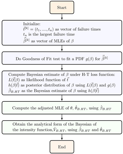
Algorithm 2. Estimate of the intensity function using Crow data in Table 1.

3.3. Sensitivity Analysis: Prior and Loss Function

To answer the second research question, “Is the Bayesian estimate of the intensity function, $V\left(t\mathrm{<mo>\; ;\; </mo>}\beta \mathrm{,}\theta \right)$, of the PLP sensitive to the selections of the prior (both parametric and non-parametric priors) and loss function?”, we developed a simulation procedure, Algorithm 3, given below.

The algorithm compares the Bayesian and MLE estimates of the intensity function, $V\left(t\mathrm{<mo>\; ;\; </mo>}\beta \mathrm{,}\theta \right)$, under different prior PDFs, for various sample sizes, with the H-T and S-E loss functions. The relative efficiency is used to compare these estimates of the $V\left(t\mathrm{<mo>\; ;\; </mo>}\beta \mathrm{,}\theta \right)$. The relative efficiency with a value less than 1, larger than 1, and approximately equal to 1 indicate that the Bayesian estimates under the H-T loss function are more, less, equally efficient to the Bayesian estimate under the S-E loss function and the same analysis is applied when we compared to the MLE of $V\left(t\mathrm{<mo>\; ;\; </mo>}\beta \mathrm{,}\theta \right)$, respectively. The algorithm starts by initializing the shape and scale parameters of the PLP, $\beta$ and $\theta$, respectively, and the number of iterations p.

Algorithm 3. Simulation to compare Bayesian and MLE estimates of the intensity function. Notations found in Table 2.

For various sample sizes ( $n=20,40,80,140$ ), random failure times (time to failures) distributed according to the PLP are simulated using the initialized values of the PLP parameters. Then, the Bayesian and MLE estimates of the key parameter $\beta$ are computed and used to compute the Bayesian estimates of $\theta$, respectively. After a predetermined number of iterations, the average values of the Bayesian and MLE estimates of $\beta$ and $\theta$ were used to obtain the analytical forms of the $V\left(t\mathrm{<mo>\; ;\; </mo>}\beta \mathrm{,}\theta \right)$ under Bayesian, for both H-T and S-E loss functions and MLE, namely ${\hat{V}}_{HT}\mathrm{,}{\hat{V}}_{SE}$, and ${\hat{V}}_{MLE}$, respectively. Informative parametric priors were considered such as the inverted gamma and the Burr PDFs, whereas the Jeffery prior was chosen as non-informative prior. In addition, probability kernel density function is selected as a non-parametric prior PDF. Probability kernel density estimation depends on the sample size, bandwidth, and the choice of the kernel function ( $K\left(u\right)$ ). In this study, the optimal bandwidth ( $h^{\mathrm{<mo>\; *\; </mo>}}$ ) and kernel function were chosen to minimize the asymptotic mean integrated squared error (AMISE). The simplified form of the AMISE is reduced to:

$\text{AMISE}\left(\hat{f}\left(\beta \right)\right)=\frac{C\left(K\right)}{n\cdot h}+\left(\frac{1}{4}\cdot h^4\cdot k_2^2\cdot R\left(f^{\left(2\right)}\left(\beta \right)\right)\right)$ (47)

where:

Ÿ $C\left(K\right)={\displaystyle \int }{\left(K\left(u\right)\right)}^2\text{d}u$.

Ÿ n: sample size.

Ÿ h: bandwidth.

Ÿ $k_2={\displaystyle {\int }_{-\infty }^{+\infty }}{u}^2\cdot K\left(u\right)\text{d}u$.

Ÿ $f^{\left(2\right)}\left(\beta \right)$ is the second derivative of Burr PDF.

Ÿ $R\left(f^{\left(2\right)}\left(\beta \right)\right)={\displaystyle \int }{\left(f^{\left(2\right)}\left(\beta \right)\right)}^2\text{d}\beta$.

Ÿ $h^{*}={\left[\frac{C\left(K\right)}{k_2^2\cdot R\left(f^{\left(2\right)}\left(\beta \right)\right)}\right]}^{1/5}\cdot n^{-1/5}$.

AMISE was numerically calculated using the optimal bandwidth, with respect to different samples sizes for each kernel function considered in this study, namely Epanechnikov, Cosine, Biweight, Triweight, Gaussian, Triangle, Uniform, Tricube, and Logistic kernel functions. The results is given by Table 10.

The minimum AMISE corresponds to the Epanechnikov kernel function ( $K\left(u\right)=\frac{3}{4}\left(1-u^2\right)I_{\left|u\right|\le 1}$ ). In addition to the Epanechnikov kernel function, the Gaussian kernel function ( $K\left(u\right)=\frac{1}{\sqrt{2\text{π}}}\exp \left(\frac{-u^2}{2}\right)I_{\mathbb{I}\text{}R}$ ) was also used in the calculation since it is commonly used for its analytical tractability.

Numerical integration techniques were used to compute the Bayesian estimates of the intensity function, $V\left(t\mathrm{<mo>\; ;\; </mo>}\beta \mathrm{,}\theta \right)$, parameters under both H-T and S-E loss functions according to the equations defined in Section 2.3, for each of the parametric and non-parametric prior PDFs. Samples of size 20, 40, 80, and

Table 10. Calculations of the AMISE with respect to different sample size, optimal bandwidth, and kernel function.

140 were generated where the parameters $\beta$ and $\theta$ were initialized to be 0.7054 and 1.7441, respectively. In the analytical form (17), $f_1$ and $f_2$ are conditioned to be positive numbers and play a big role in assigning the weight of loss depending on the estimator’s behavior, whether underestimating or overestimating. Therefore, the simulation procedure was repeated three times according to the following cases:

1) $f_1>f_2$

2) $f_1<f_2$

3) $f_1=f_2$

The results for 1000 repetitions, $f_1>f_2$, and $n=20,40,80,140$, are shown in Table 11.

It can be observed that the Bayesian estimate of the $V\left(t\mathrm{<mo>\; ;\; </mo>}\beta \mathrm{,}\theta \right)$ under the H-T loss function ( ${\hat{V}}_{HT}$ ) and S-E loss function ( ${\hat{V}}_{SE}$ ) had an outstanding efficiency compared to the MLE of the $V\left(t\mathrm{<mo>\; ;\; </mo>}\beta \mathrm{,}\theta \right)$ ( ${\hat{V}}_{MLE}$ ) for all sample sizes and prior PDFs, with the exception of the sample sizes 20 and 40 when inverted gamma PDF was the selected prior. The ${\hat{V}}_{HT}$ was more efficient (6% - 11% estimation improvement) compared to the ${\hat{V}}_{SE}$ when Burr PDF is selected to be the prior. The ${\hat{V}}_{HT}$ had similar efficiency compared to the ${\hat{V}}_{SE}$ when Jeffrey prior is selected and for large sample sizes, whereas unsurprisingly ${\hat{V}}_{SE}$ was more efficient for small sample sizes since Jeffrey Bayesian estimate of the key parameter $\beta$ tends to overestimate and for the H-T loss function gives more exponential weight on the extreme overestimate loss than the extreme under-estimate loss when $f_1>f_2$. For Bayesian Gaussian and Epanechnikov kernel estimates, the ${\hat{V}}_{HT}$ was more efficient compared to the ${\hat{V}}_{SE}$ for sample sizes $n=20,40$ and 80 with 11% - 13% of estimation improvement even though they tend to underestimate and the H-T loss function puts more exponential weight on the extreme underestimation, but tend to have similar efficiency for sample size $n=140$.

Table 11. The relative efficiency (RE) of the Bayesian estimate under H-T loss function, ${\hat{V}}_{HT}$ when $f_1>f_2$, compared to the Bayesian estimate under S-E loss function, ${\hat{V}}_{SE}$, and the MLE, ${\hat{V}}_{MLE}$, of $V\left(t\mathrm{<mo>\; ;\; </mo>}\beta \mathrm{,}\theta \right)$.

The results for 1000 repetitions, $f_1>f_2$, and $n=20,40,80,140$, are shown in Table 12.

Again, the Bayesian MLE estimate of the $V\left(t\mathrm{<mo>\; ;\; </mo>}\beta \mathrm{,}\theta \right)$ under the H-T loss function ( ${\hat{V}}_{HT}$ ) and S-E loss function ( ${\hat{V}}_{SE}$ ) had an outstanding efficiency compared to the MLE of the $V\left(t\mathrm{<mo>\; ;\; </mo>}\beta \mathrm{,}\theta \right)$ ( ${\hat{V}}_{MLE}$ ) for all sample sizes and prior PDFs. When the inverted gamma was selected as prior, the ${\hat{V}}_{HT}$ was more efficient compared to the ${\hat{V}}_{SE}$ for all sample sizes with an approximately 2% of estimation improvement. As expected, the ${\hat{V}}_{HT}$ was less efficient compared to the ${\hat{V}}_{SE}$ when Burr PDF, and Gaussian and Epanechnikov kernel densities are selected as priors for sample sizes 20 and 40, since they tend to underestimate the $V\left(t\mathrm{<mo>\; ;\; </mo>}\beta \mathrm{,}\theta \right)$ parameters, and the H-T loss function tends to put more weight on the extreme overestimation than on the extreme underestimation when $f_1>f_2$. But the ${\hat{V}}_{HT}$ and ${\hat{V}}_{SE}$ had approximately similar efficiency for sample size $n=80$, and the ${\hat{V}}_{HT}$ tends to be slightly more efficient for large sample size ( $n=140$ ). The ${\hat{V}}_{HT}$ was more efficient (4% - 24% estimation

Table 12. The relative efficiency (RE) of the Bayesian estimate under H-T loss function, ${\hat{V}}_{HT}$ when $f_1<f_2$, compared to the Bayesian estimate under S-E loss function, ${\hat{V}}_{SE}$, and the MLE, ${\hat{V}}_{MLE}$, of $V\left(t\mathrm{<mo>\; ;\; </mo>}\beta \mathrm{,}\theta \right)$.

improvement) compared to the ${\hat{V}}_{SE}$ when Burr Jeffrey is chosen to be the prior PDF. The ${\hat{V}}_{HT}$ had similar efficiency compared to the ${\hat{V}}_{SE}$ for large sample sizes and when Jeffrey prior is selected, whereas unsurprisingly ${\hat{V}}_{SE}$ was more efficient for small sample sizes since Jeffrey Bayesian estimate of the key parameter $\beta$ tends to overestimate and for the H-T loss function gives more exponential weight on the extreme overestimate loss than the extreme under-estimate loss when $f_1>f_2$. For Bayesian Gaussian and Epanechnikov kernel estimates, the ${\hat{V}}_{HT}$ was more efficient compared to the ${\hat{V}}_{SE}$ for sample sizes $n=20,40$ and 80 with 11% - 13% of estimation improvement even though they tend to underestimate and the H-T loss function puts more exponential weight on the extreme underestimation, but tend to have similar efficiency for sample size $n=140$.

The results for 1000 repetitions, $f_1>f_2$, and $n=20,40,80,140$, are shown in Table 13.

Table 13. The relative efficiency (RE) of the Bayesian estimate under H-T loss function, ${\hat{V}}_{HT}$ when $f_1=f_2$, compared to the Bayesian estimate under S-E loss function, ${\hat{V}}_{SE}$, and the MLE, ${\hat{V}}_{MLE}$, of $V\left(t\mathrm{<mo>\; ;\; </mo>}\beta \mathrm{,}\theta \right)$.

Again, the Bayesian MLE estimate of the $V\left(t\mathrm{<mo>\; ;\; </mo>}\beta \mathrm{,}\theta \right)$ under the H-T loss function ( ${\hat{V}}_{HT}$ ) and S-E loss function ( ${\hat{V}}_{SE}$ ) had an outstanding efficiency compared to the MLE of the $V\left(t\mathrm{<mo>\; ;\; </mo>}\beta \mathrm{,}\theta \right)$ ( ${\hat{V}}_{MLE}$ ) for all sample sizes and prior PDFs, with the exception of the sample sizes 20 and 40 when inverted gamma PDF was the selected prior. It is observed that both ${\hat{V}}_{HT}$ and ${\hat{V}}_{SE}$ had similar efficiency in estimation of the $V\left(t\mathrm{<mo>\; ;\; </mo>}\beta \mathrm{,}\theta \right)$ for all sample sizes and priors considered in this study.

The sensitivity analysis shows that the Bayesian estimates of the intensity function of the PLP is sensitive to the prior and loss function selections. Tables 11-13 indicate the efficiency of the Bayesian estimates under the H-T loss function when compared to the Bayesian estimate under S-E loss function and to the MLE, given that the engineer should choose the values of $f_1$ and $f_2$ based on his/her estimator’s behaviour (underestimating and over estimating). Moreover, $f_1>f_2$ is the recommended choice when the engineer selects Burr or kernel PDFs as their prior knowledge of the behavior of the key parameter $\beta$. On the other hand, if the engineer does not have a prior knowledge of the key parameter $\beta$, it is still recommended to use H-T loss function in the Bayesian calculations with $f_1<f_2$.

Thus far, we showed the more accuracy in estimating a software reliability when applying the Bayesian analysis under the H-T loss function compared to the Bayesian analysis under the S-E loss function and the MLE of the subject analysis. The performed extensive analysis requires efficiency in utilizing the existing programming languages, which therefore requires some programming experience, we developed an interactive user interface application using Wolfram language to compute and visualize the Bayesian and maximum likelihood estimates of the intensity and reliability functions of the Power Law Process for a given data.

4. Conclusions

In the present study, we developed the analytical Bayesian estimates of the key parameter $\beta$, under Higgin-Tsokos and squared-error loss functions, in the intensity function where the underlying failure distribution is the Power Law Process, that is used for software reliability assessment, among others. The reliability function of the subject model is written analytically as a function of the intensity function.

The behavior of the key parameter $\beta$ is characterized by the Burr type XII probability distribution. Real data and numerical simulation were used to illustrate not only the robustness of the squared-error loss function being challenged by the assumption of the Higgins-Tsokos loss function, but also the efficiency improvement in the estimation of the intensity function of PLP under Higgins-Tsokos loss function ( ${\hat{V}}_{B\mathrm{.}HT}\left(t\right)$ ). For 100,000 samples of software failure times, based on Monte Carlo simulations and sample size of 40, the Bayesian estimate of $\beta$ under Higgins-Tsokos loss function ( ${\hat{\beta }}_{B\mathrm{.}HT}$ ) performed slightly better than the Bayesian estimate of $\beta$ under squared-error loss function ( ${\hat{\beta }}_{B\mathrm{.}SE}$ ) with respect to three different values of $\theta$ (0.5, 1.7441, 4). Even for different sample sizes (20, 30, 40, 50, 60, 70, 80, 100, 120, 140, and 160), similar results were achieved using $\beta =0.7054$, $\theta =1.7441$, and averaged over 10,000 samples of software failure times.

As the MLE of the second parameter in the intensity function ( $\theta$ ) depends on the estimate of $\beta$, the adjusted estimate of $\theta$ ${\hat{\beta }}_{B\mathrm{.}HT}$ provided better performance compared to the adjusted estimate of $\theta$ using the ${\hat{\beta }}_{B\mathrm{.}SE}\left(t\right)$. Moreover, the Relative Efficiency was used to compare the intensity function estimations, mainly using MLEs for both $\beta$ and $\theta$ ( ${\hat{V}}_{MLE}\left(t\right)$ ), using Bayesian estimate of $\beta$ under the squared-error loss function and Bayesian of $\theta$ ( ${\hat{V}}_{B\mathrm{.}SE}\left(t\right)$ ), and using Bayesian estimate of $\beta$ under the Higgins-Tsokos loss function and Bayesian of $\theta$ ( ${\hat{V}}_{B\mathrm{.}HT}\left(t\right)$ ), showing that ${\hat{V}}_{B\mathrm{.}HT}\left(t\right)$ is more efficient in estimating the intensity function $V\left(t\right)$ with about 12% estimation improvement.

With respect to the question: Is the Bayesian estimate of the intensity function, $V\left(t\mathrm{<mo>\; ;\; </mo>}\beta \mathrm{,}\theta \right)$, of the PLP sensitive to the selections of the prior, both parametric and non-parametric priors, and loss function? The parametric prior PDFs were Burr, Jeffrey, and inverted gamma probability distributions whereas the non-parametric priors were Gaussian and Epanechnikov kernel densities. The priors’ parameters were estimated using Crow failure times. Additionally, the optimal bandwidth and kernel functions were selected to minimize the asymptotic mean integrated squared error.

Using the developed algorithm, 1000 samples of software failure times with respect to four sample sizes of n (20, 40, 80, and 140) were generated from the PLP to compare the Bayesian estimates of $V\left(t\mathrm{<mo>\; ;\; </mo>}\beta \mathrm{,}\theta \right)$ under the subject priors and loss functions using the Relative Efficiency among them. The simulation procedure was repeated three times for the cases when $f_1>f_2$, $f_1<f_2$, and $f_1=f_2$. The results showed the efficacy of the Bayesian estimates of H-T loss function, and the choice of the $f_1$ and $f_2$ values depends on the prior knowledge of the key parameter $\beta$. It is recommended to choose values where $f_1>f_2$ when the engineer thinks the prior knowledge of $\beta$ is best characterized by Burr or Kernel based probability distributions with a proper justification, whereas a choice of $f_1<f_2$ and Jeffery’s prior is suggested when the engineer does not have a prior knowledge of $\beta$.

Thus, based on this aspect of our analysis, we can conclude that the Bayesian analysis approach under Higgins-Tsokos loss function not only as robust as the Bayesian analysis approach under squared error loss function but also performed better, where both are superior to the maximum likelihood approach in estimating the reliability function of the Power Law Process. The interactive user interface application can be used without any prior coding knowledge to compute and visualize the Bayesian and maximum likelihood estimates of the intensity and reliability functions of the Power Law Process for a given data.

Acknowledgements

We thank Majmaah University for funding the research, along with the support provided by the University of South Florida.

Conflicts of Interest

The authors declare no conflicts of interest regarding the publication of this paper.

References

[1]	Duane, J.T. (1964) Learning Curve Approach to Reliability Monitoring. IEEE Transactions on Aerospace, 2, 563-566. https://doi.org/10.1109/TA.1964.4319640
[2]	Crow, L.H. (1975) Tracking Reliability Growth. Proceedings of the 20th Conference on Design of Experiments, Report 75-2, US Army Research Office, Research Triangle Park, NC, 741-754.
[3]	Yamada, S., Ohba, M. and Osaki, S. (1983) S-Shaped Reliability Growth Modeling for Software Error Detection. IEEE Transactions on Reliability, R-32, 475-484. https://doi.org/10.1109/TR.1983.5221735
[4]	Goel, A.L. and Okumoto, K. (1979) Time-Dependent Error-Detection Rate Model for Software Reliability and Other Performance Measures. IEEE Transactions on Reliability, R-28, 206-211. https://doi.org/10.1109/TR.1979.5220566
[5]	Calabria, R., Guida, M. and Pulcini, G. (1992) A Bayes Procedure for Estimation of Current System Reliability. IEEE Transactions on Reliability, 41, 616-620. https://doi.org/10.1109/24.249599
[6]	Bain, L. and Engelhardt, M. (1991) Statistical Analysis of Reliability and Life Testing Models. Marcel-Dekker, New York, NY, USA,.
[7]	Goel, A.L. and Okumoto, K. (1984) Bayesian Inference for the Weibull Process with Applications to Assessing Software Reliability Growth and Predicting Software Failures. Proc. Sixteenth Symp. Interface, R-28, 206-211.
[8]	Tsokos, C.P. and Rao, A.N.V. (1994) Estimation of Failure Intensity for the Weibull Process. Reliability Engineering & System Safety, 45, 271–275. https://doi.org/10.1016/0951-8320(94)90143-0
[9]	Rigdon, S.E. and Basu, A.P. (1989) The Effect of Assuming a Homogeneous Poisson Process when the True Process Is a Power Law Process. Journal of Quality Technology, 22, 111-117. https://doi.org/10.1080/00224065.1990.11979222
[10]	Rigdon, S.E. and Basu, A.P. (1989) The Power Law Process: A Model for the Reliability of Repairable Systems. Journal of Quality Technology, 21, 251-260. https://doi.org/10.1080/00224065.1989.11979183
[11]	Rigdon, S.E. and Basu, A.P. (1990) Estimating the Intensity Function of a Power Law Process at the Current Time: Time Truncated Case. Communications in Statistics—Simulation and Computation, 19, 1079-1104. https://doi.org/10.1080/03610919008812906
[12]	Luo, L., Xing, L. and Levitin, G. (2018) Optimizing Dynamic Survivability and Security of Replicated Data in Cloud Systems under Co-Residence Attacks. Reliability Engineering & System Safety, in press. https://doi.org/10.1016/j.ress.2018.09.014
[13]	Movahedi, Y., Cukier, M., Andongabo, A. and Gashi, I. (2018) Cluster-Based Vulnerability Assessment of Operating Systems and Web Browsers. 2017 13th European Dependable Computing Conference, Geneva, 4-8 September 2017, 18-25. https://doi.org/10.1109/EDCC.2017.27
[14]	Tsokos, C.P. and Xu, Y. (2011) Non-Homogenous Poisson Process for Evaluating Stage I & II Ductal Breast Cancer Treatment. Journal of Modern Applied Statistical Methods, 10, 646-655. https://doi.org/10.22237/jmasm/1320121320
[15]	But, A., Härkänen, T. and Haukka, J. (2017) Non-Parametric Bayesian Intensity Model: Exploring Time-to-Event Data on Two Time Scales. Scandinavian Journal of Statistics, 44, 798-814, June. https://doi.org/10.1111/sjos.12280
[16]	Turnbull, B.W., Abu-Libdeh, H. and Clark, L.C. (1990) Estimation of Failure Intensity for the Weibull Process. Biometrics, 46, 1017-1034. https://doi.org/10.2307/2532445
[17]	Raberto, M., Scalas, E., Ponta, L., Trinh, M. and Cincotti, S. (2019) Modeling Non-Stationarities in High-Frequency Financial Time Series. Physica A: Statistical Mechanics and Its Applications, 521, 173-196. https://doi.org/10.1016/j.physa.2019.01.069
[18]	Kieu, L.M. (2018) Analytical Modelling of Point Process and Application to Transportation. In: Zhou, J. and Chen, F., Eds., Human and Machine Learning. Human–Computer Interaction Series, Springer, Cham. https://doi.org/10.1007/978-3-319-90403-0_19
[19]	Sayarshad, H.R. and Chow, J.Y.J. (2016) Survey and Empirical Evaluation of Nonhomogeneous Arrival Process Models with Taxi Data. Journal of Advanced Transportation, 50, 1275-1294. https://doi.org/10.1002/atr.1401
[20]	Qi, G., Pan, G., Li, S., Wu, Z., Zhang, D., Sun, L. and Yang, L.T. (2013) How Long a Passenger Waits for a Vacant Taxi—Large-Scale Taxi Trace Mining for Smart Cities. 2013 IEEE International Conference on Green Computing and Communications and IEEE Internet of Things and IEEE Cyber, Physical and Social Computing, Beijing, 20-23 August 2013, 1029-1036. https://doi.org/10.1109/GreenCom-iThings-CPSCom.2013.175
[21]	Menon, A.K. and Lee, Y. (2017) Predicting Short-Term Public Transport Demand via Inhomogeneous Poisson Processes. In: Proceedings of the 2017 ACM on Conference on Information and Knowledge Management, ACM, New York, 2207-2210.
[22]	Yue, D., Zhao, G. and Yue, W. (2016) Analysis of a Multi-Server Queueing-Inventory System with Non-Homogeneous Poisson Arrivals. In: Proceedings of the 11th International Conference on Queueing Theory and Network Applications, ACM, New York.
[23]	Kimura, M., Toyota, T. and Yamada, S. (1999) Economic Analysis of Software Release Problems with Warranty Cost and Reliability Requirement. Reliability Engineering & System Safety, 66, 49-55. https://doi.org/10.1016/S0951-8320(99)00020-4
[24]	Molinares, C.A. and Tsokos, C.P. (2013) Bayesian Reliability Approach to the Power Law Process with Sensitive Analysis to Prior Selection. International Journal of Reliability, Quality and Safety Engineering, 20, No. 1. https://doi.org/10.1142/S0218539313500046
[25]	Alenezi, F.N. and Tsokos, C.P. (2018) Bayesian Reliability Analysis of the Power Law Process with Respect to the Higgins-Tsokos Loss Function for Modeling Software Failure Times. Submitted for Publication.
[26]	Higgins, J.J. and Tsokos, C.P. (1980) A Study of the Effect of the Loss Function on Bayes Estimates of Failure Intensity, MTBF, and Reliability. Applied Mathematics and Computation, 6, 145-166. https://doi.org/10.1016/0096-3003(80)90039-9
[27]	Crow, L.H. (1975) Reliability Analysis for Complex, Repairable Systems. In: Proschan, F. and Serfling, D.J., Eds., Reliability and Biometry, Society for Industrial and Applied Mathematics, Philadelphia, PA, 379-410.
[28]	Jeffreys, H. (1946) An Invariant Form for the Prior Probability in Estimation Problems. Proceedings of the Royal Society of London. Series A: Mathematical and Physical Sciences, 186, 453-461. https://doi.org/10.1098/rspa.1946.0056