New Soliton Solutions to the Initial Value Problem for the Two-Component Short Pulse Equation

Yan Luo

College of Science, University of Shanghai for Science and Technology, Shanghai, China.

DOI: 10.4236/jamp.2019.71002                

Abstract

We formulate a matrix Riemann-Hilbert problem to the initial value problem for the two-component system proposed by Matsuno. By solving the associated Riemann-Hilbert problem, we can get the soliton solutions of the two-component system. One and two soliton solutions are investigated in detail.

Keywords

Riemann-Hilbert Problem, Two-Component Short Pulse Equation, Soliton Solutions

1. Introduction

The SP (short pulse) equation

$u_{xt}=u+\frac{1}{6}{\left(u^3\right)}_{xx},$ (1)

where $u=u\left(x,t\right)$ represents the magnitude of the electric field and subscripts x and t appended to u denote partial differentiation, has been proposed as a model equation describing the propagation of ultrashort optical pulses in nonlinear media [1] . A numerical analysis shows that as the pulse length shortens, the SP equation becomes a better approximation to the solution of the Maxwell equation when compared with the prediction of the NLS equation [2] . Then Matsuno proposed a novel multi-component generalization of the SP equation [3] , which generalizes the SP equation describing the propagation of ultra-short pulses in optical fibers. Here we consider the multi-component system [3] .

$u_{i,xt}=u_i+\frac{1}{2}{\left(u_{i,x}{\displaystyle \underset{j=1}{\overset{n}{\sum }}{u}_j^2}\right)}_x,i=1,2,\cdots ,n$ (2)

with reduced two-component short pulse system if letting n = 2, which given by

$\{\begin{array}{l}{u}_{xt}=u+\frac{1}{2}{\left[\left(u^2+v^2\right)u_x\right]}_x\\ v_{xt}=v+\frac{1}{2}{\left[\left(u^2+v^2\right)v_x\right]}_x\end{array}$ (3)

where $u=u_1$ and $v=u_2$ . Then we make the transformation $\left(u,v\right)\to \left(\frac{u+v}{2},\frac{u-v}{2i}\right)$ and this system can be written as

$\{\begin{array}{l}{u}_{xt}=u+\frac{1}{2}{\left(uv{u}_x\right)}_x\\ v_{xt}=v+\frac{1}{2}{\left(uv{v}_x\right)}_x\end{array}$ (4)

We named Equation (4) as 2SPE (two-component system). Obviously if we put $u=v$ , then 2SPE reduces to the SP equation. The integrability, soliton solutions, and other features of Equation (1) and Equation (4) common to the completely integrable PDEs (partial differential equations) have been studied from various points of view [3] [4] [5] [6] . And the semi-discretization of a multi-component SP equation was studied in [7] , super extensions in [8] .

Here, in this paper, we consider the initial value problem for the 2SPE (4) with the initial value data $u\left(x,t=0\right)=u_0\left(x\right)\in S\left(R\right)$ , $v\left(x,t=0\right)=v_0\left(x\right)\in S\left(R\right)$ and $S\left(R\right)$ denotes the Schwartz space. The present paper is devoted to analyze the IVP (initial value problem) for the Equation (4) by Riemann-Hilbert approach.

Organization of the paper: In Section 2, we formulate the associated Riemann-Hilbert problem by performing the similar spectral analysis to the Equation (4) as [9] . In Section 3, to obtain the soliton solutions of the Equation (4), we need analyze the residue conditions of the Riemann-Hilbert problem. Especially, the one and two soliton solutions are investigated in detail.

2. Riemann-Hilbert Problem for the Two-Component System

The 2SPE admits a WKI (Wadati-Konno-Ichikawa)-type Lax pair as follow:

$\{\begin{array}{l}{\phi }_x=X\left(x,t,k\right)\phi \\ {\phi }_t=T\left(x,t,k\right)\phi \end{array}$ (5)

where

$X=ik{X}_1,T=\frac{ik}{2}uv{X}_1+\frac{1}{4ik}{\sigma }_3-\frac{i}{2}\left(\begin{array}{cc}u& 0\\ 0& v\end{array}\right){\sigma }_2$ (6)

with

$X_1=\left(\begin{array}{cc}1& u_x\\ v_x& -1\end{array}\right),{\sigma }_3=\left(\begin{array}{cc}1& 0\\ 0& -1\end{array}\right),{\sigma }_2=\left(\begin{array}{cc}0& -i\\ i& 0\end{array}\right).$ (7)

2.1. Spectral Analysis for k = 0

Introducing

$\phi \left(x,t,k\right)={\mu }^0\left(x,t,k\right){\text{e}}^{\left(ikx+\frac{t}{4ik}\right){\sigma }_3}$ (8)

Then we can get the Lax pair of ${\mu }^0$

$\{\begin{array}{l}{\mu }_x^0-ik\left[{\sigma }_3,{\mu }^0\right]=V_1^0{\mu }^0\\ {\mu }_t^0-\frac{1}{4ik}\left[{\sigma }_3,{\mu }^0\right]=V_2^0{\mu }^0\end{array}$ (9)

where

$V_1^0=ik\left(\begin{array}{cc}0& u_x\\ v_x& 0\end{array}\right),V_2^0=\left(\begin{array}{cc}\frac{ik}{2}uv& \frac{ik}{2}uv{u}_x-\frac{u}{2}\\ \frac{ik}{2}uv{v}_x+\frac{v}{2}& -\frac{ik}{2}uv\end{array}\right)$ (10)

We define two eigenfunctions of ${\mu }_j^0\left(x,t,k\right)$

$\{\begin{array}{l}{\mu }_1^0\left(x,t,k\right)=I+{\displaystyle {\int }_{-\infty }^x{\text{e}}^{ik\left(x-y\right){\sigma }_3}{V}_1^0\left(y,t,k\right){\text{e}}^{-ik\left(x-y\right){\sigma }_3}{\mu }_1^0\left(y,t,k\right)\text{d}y}\\ {\mu }_2^0\left(x,t,k\right)=I-{\displaystyle {\int }_x^{+\infty }{\text{e}}^{ik\left(x-y\right){\sigma }_3}{V}_1^0\left(y,t,k\right){\text{e}}^{-ik\left(x-y\right){\sigma }_3}{\mu }_2^0\left(y,t,k\right)\text{d}y}\end{array}$ (11)

Proposition 1: The functions ${\left\{{\mu }_j^0\right\}}_1^2$ are bounded and analytic as:

${\mu }_1^0\in \left(D_2,D_1\right),{\mu }_2^0\in \left(D_1,D_2\right).$ (12)

where $\left[{\mu }_j^0\right]\in \left(D_2,D_1\right)$ means that the 1-th column ${\left[{\mu }_j^0\right]}_1$ and 2-th column ${\left[{\mu }_j^0\right]}_2$ of ${\mu }_j^0$ are bounded and analytic in $D_2$ and $D_1$ , respectively, $D_1=\left\{k\in ℂ|\mathrm{Im}k>0\right\}$ and $D_2=\left\{k\in ℂ|\mathrm{Im}k<0\right\}.$

Proposition 2: The functions ${\mu }_j^0\left(x,t,k\right)$ have the expansions as:

${\mu }_j^0\left(x,t,k\right)=I+\left(\begin{array}{cc}0& iu\\ iv& 0\end{array}\right)k+O\left(k^2\right),k\to 0.$ (13)

2.2. Spectral Analysis for k = ∞

Define

$G\left(x,t\right)=\sqrt{\frac{\sqrt{m}+1}{2\sqrt{m}}}\left(\begin{array}{cc}1& -\frac{\sqrt{m}-1}{v_x}\\ \frac{\sqrt{m}-1}{u_x}& 1\end{array}\right),$ (14)

$p\left(x,t,k\right)=x-{\displaystyle {\int }_x^{\infty }\left(\sqrt{m\left(x^{\prime },t\right)}-1\right)\text{d}{x}^{\prime }}-\frac{t}{4k^2},$ (15)

where $m=1+u_x{v}_x$ .

Introduce the following transformation:

$\phi \left(x,t,k\right)=G\left(x,t\right){\text{e}}^{h_{-}{\sigma }_3}\mu \left(x,t,k\right){\text{e}}^{-h_{-}{\sigma }_3}{\text{e}}^{-h_{+}{\sigma }_3}{\text{e}}^{ikp\left(x,t,k\right){\sigma }_3}$ (16)

where

$h_{-}={\displaystyle {\int }_{-\infty }^x\frac{u_x{v}_{xx}-u_{xx}{v}_x}{4\sqrt{m}\left(\sqrt{m}+1\right)}\left(x^{\prime },t\right)\text{d}{x}^{\prime }},$ (17)

$h_{+}={\displaystyle {\int }_x^{+\infty }\frac{u_x{v}_{xx}-u_{xx}{v}_x}{4\sqrt{m}\left(\sqrt{m}+1\right)}\left(x^{\prime },t\right)\text{d}{x}^{\prime }},$ (18)

$h=h_{+}+h_{-}={\displaystyle {\int }_{-\infty }^{+\infty }\frac{u_x{v}_{xx}-u_{xx}{v}_x}{4\sqrt{m}\left(\sqrt{m}+1\right)}\left(x^{\prime },t\right)\text{d}{x}^{\prime }}.$ (19)

We find the Lax pair equation of $\mu \left(x,t,k\right)$

$\{\begin{array}{l}{\mu }_x-ik{p}_x\left[{\sigma }_3,\mu \right]=V_1\mu \\ {\mu }_t-ik{p}_t\left[{\sigma }_3,\mu \right]=V_2\mu \end{array}$ (20)

where

$V_1=-\left(\begin{array}{cc}0& -\frac{\left(\sqrt{m}+1\right)m_x}{4m{v}_x}+\frac{u_x{v}_{xx}}{2\sqrt{m}{v}_x}\\ \frac{\left(\sqrt{m}+1\right)m_x}{4m{u}_x}-\frac{u_{xx}{v}_x}{2\sqrt{m}{u}_x}& 0\end{array}\right)$ (21)

$\begin{array}{c}{V}_2=\frac{1}{4ik}\left(\frac{1}{\sqrt{m}}-1\right){\sigma }_3-\frac{1}{4ik}\cdot \frac{1}{\sqrt{m}}\left(\begin{array}{cc}0& u_x\\ v_x& 0\end{array}\right)\\ +\frac{1}{4\sqrt{m}}\left(\begin{array}{cc}0& -\frac{\left(\sqrt{m}-1\right)u_{x}v+\left(\sqrt{m}+1\right)u{v}_x}{v_x}\\ \frac{\left(\sqrt{m}+1\right)u_{x}v+\left(\sqrt{m}-1\right)u{v}_x}{u_x}& 0\end{array}\right)\\ \cdot \left(\begin{array}{cc}0& -\frac{\left(\sqrt{m}+1\right)m_x}{4m{v}_x}+\frac{u_x{v}_{xx}}{2\sqrt{m}{v}_x}\\ \frac{\left(\sqrt{m}+1\right)m_x}{4m{u}_x}-\frac{u_{xx}{v}_x}{2\sqrt{m}{u}_x}& 0\end{array}\right)\end{array}$ (22)

Then, define two eigenfunctions of ${\mu }_j\left(x,t,k\right)$ :

$\{\begin{array}{l}{\mu }_1=I+{\displaystyle {\int }_{-\infty }^x{\text{e}}^{ik\left[p\left(x,t,k\right)-p\left(y,t,k\right)\right]{\sigma }_3}{V}_1\left(y,t,k\right){\text{e}}^{ik\left[p\left(x,t,k\right)-p\left(y,t,k\right)\right]{\sigma }_3}{\mu }_1\left(y,t,k\right)\text{d}y}\\ {\mu }_2=I-{\displaystyle {\int }_x^{+\infty }{\text{e}}^{ik\left[p\left(x,t,k\right)-p\left(y,t,k\right)\right]{\sigma }_3}{V}_1\left(y,t,k\right){\text{e}}^{ik\left[p\left(x,t,k\right)-p\left(y,t,k\right)\right]{\sigma }_3}{\mu }_2\left(y,t,k\right)\text{d}y}\end{array}$ (23)

Proposition 3: The functions ${\left\{{\mu }_j\right\}}_1^2$ are bounded and analytic as:

${\mu }_1\in \left(D_2,D_1\right),{\mu }_2\in \left(D_1,D_2\right).$ (24)

Proposition 4: The functions ${\mu }_j\left(x,t,k\right)$ also satisfies

${\mu }_j\left(x,t,k\right)=I+O\left(\frac{1}{k}\right),k\to \infty .$ (25)

Proposition 5: (Symmetry property) In this paper, we consider the function $u\left(x,t\right)$ and $v\left(x,t\right)$ are real-value functions. Then, the eigenfunctions ${\mu }_j\left(x,t,k\right)$ satisfy the following symmetry property:

$\overline{{\mu }_j\left(-\stackrel{¯}{k}\right)}={\mu }_j\left(k\right)$ (26)

2.3. Spectral Function s(k)

The eigenfunctions ${\mu }_1\left(x,t,k\right)$ and ${\mu }_2\left(x,t,k\right)$ are related

${\mu }_1\left(x,t,k\right)={\mu }_2\left(x,t,k\right){\text{e}}^{ikp\left(x,t,k\right){\sigma }_3}s\left(k\right){\text{e}}^{-ikp\left(x,t,k\right){\sigma }_3}$ (27)

where the matrix $s\left(k\right)$ is independent of $\left(x,t\right)$ and has the form

$s\left(k\right)=\left(\begin{array}{cc}a\left(k\right)& b\left(k\right)\\ c\left(k\right)& d\left(k\right)\end{array}\right)$ (28)

The function $a\left(k\right)$ and $d\left(k\right)$ can be computed by

$\{\begin{array}{l}a\left(k\right)=\det \left(\begin{array}{cc}{\left[{\mu }_1\right]}_1& {\left[{\mu }_2\right]}_2\end{array}\right)\\ d\left(k\right)=\det \left(\begin{array}{cc}{\left[{\mu }_2\right]}_1& {\left[{\mu }_1\right]}_2\end{array}\right)\end{array}$ (29)

where $\det \left(X\right)$ means the determinate of matrix X.

Hence, form the analytic properties of the functions ${\mu }_j$ , we know that $d\left(k\right)$ and $a\left(k\right)$ are analytic in $D_1$ and $D_2$ , respectively.

2.4. The Relation between ${\mu }_j\left(x,t,k\right)$ and ${\mu }_j^0\left(x,t,k\right)$

Proposition 6: The functions ${\mu }_j\left(x,t,k\right)$ and ${\mu }_j^0\left(x,t,k\right)$ are related

$\{\begin{array}{l}{\mu }_1\left(x,t,k\right)={\text{e}}^{-h_{-}{\sigma }_3}{G}^{-1}\left(x,t\right){\mu }_1^0\left(x,t,k\right){\text{e}}^{-ik{d}_{-}{\sigma }_3},\\ {\mu }_2\left(x,t,k\right)={\text{e}}^{-h_{-}{\sigma }_3}{G}^{-1}\left(x,t\right){\mu }_2^0\left(x,t,k\right){\text{e}}^{ik{d}_{+}{\sigma }_3}{\text{e}}^{h{\sigma }_3},\end{array}$ (30)

where $d_{-}={\displaystyle {\int }_{-\infty }^x\left(\sqrt{m\left(x^{\prime },t\right)}-1\right)\text{d}{x}^{\prime }}$ and $d_{+}={\displaystyle {\int }_x^{+\infty }\left(\sqrt{m\left(x^{\prime },t\right)}-1\right)\text{d}{x}^{\prime }}$ .

Proposition 7: The spectral functions $a\left(k\right)$ and $d\left(k\right)$ have the following asymptotic behaviors as $k\to 0$ :

$\{\begin{array}{l}a\left(k\right)={\text{e}}^{-h}\left(1-ikd-\frac{d^2}{2}{k}^2+O\left(k^3\right)\right)\\ d\left(k\right)={\text{e}}^h\left(1+ikd-\frac{d^2}{2}{k}^2+O\left(k^3\right)\right)\end{array}$ (31)

where $d=d_{-}+d_{+}$ .

2.5. The Riemann-Hilbert Problem

Let us define

$M\left(x,t,k\right)=\{\begin{array}{l}\left(\begin{array}{cc}{\left[{\mu }_2\right]}_1& \frac{{\left[{\mu }_1\right]}_2}{d\left(k\right)}\end{array}\right),k\in D_1\\ \left(\begin{array}{cc}\frac{{\left[{\mu }_1\right]}_1}{a\left(k\right)}& {\left[{\mu }_2\right]}_2\end{array}\right),k\in D_2\end{array}$ (32)

Making coordinate transformation

$y\left(x,t\right)=x-{\displaystyle {\int }_x^{+\infty }\left(\sqrt{m\left(x^{\prime },t\right)}-1\right)\text{d}{x}^{\prime }}=x-d_{+}\left(x,t\right)$ (33)

and defining

$\tilde{M}\left(y,t,k\right)=M\left(x\left(y,t\right),t,k\right)$ (34)

Then, $\tilde{M}\left(y,t,k\right)$ satisfies the Riemann-Hilbert problem as follows:

${\tilde{M}}_{+}\left(y,t,k\right)={\tilde{M}}_{-}\left(y,t,k\right)J\left(y,t,k\right),k\in ℝ,$ (35)

$\tilde{M}\left(y,t,k\right)={\rm I},k\to \infty ,$ (36)

where

$J\left(y,t,k\right)={\text{e}}^{ik\left(ky-\frac{t}{4k}\right){\sigma }_3}{J}_0\left(k\right){\text{e}}^{-ik\left(ky-\frac{t}{4k}\right){\sigma }_3}.$ (37)

To obtain the solution $u\left(x,t\right)$ and $v\left(x,t\right)$ of the Equation (4), we need the asymptotic behavior of $M\left(x,t,k\right)$ as $k\to 0$ ,

$M\left(x,t,k\right)={\text{e}}^{-h_{-}{\sigma }_3}{G}^{-1}\left(x,t,k\right)\left[I+k\left(\begin{array}{cc}{d}_{+}& iu\\ iv& -d_{+}\end{array}\right)+O\left(k^2\right)\right]{\text{e}}^{h{\sigma }_3}$ (38)

Hence, we can get the solution of Equation (4)

$\{\begin{array}{l}u\left(x,t\right)=u\left(y\left(x,t\right),t\right)\\ v\left(x,t\right)=v\left(y\left(x,t\right),t\right)\end{array}$ (39)

where

$\{\begin{array}{l}x\left(y,t\right)=y+\underset{k\to 0}{\lim }\frac{{\left[\tilde{M}{\left(y,t,0\right)}^{-1}\cdot \tilde{M}\left(y,t,k\right)\right]}_{11}-1}{ik}\\ {\text{e}}^{-2h}\cdot u\left(y,t\right)=\underset{k\to 0}{\lim }\frac{{\left[\tilde{M}{\left(y,t,0\right)}^{-1}\cdot \tilde{M}\left(y,t,k\right)\right]}_{12}}{ik}\\ {\text{e}}^{2h}\cdot v\left(y,t\right)=\underset{k\to 0}{\lim }\frac{{\left[\tilde{M}{\left(y,t,0\right)}^{-1}\cdot \tilde{M}\left(y,t,k\right)\right]}_{21}}{ik}\end{array}$ (40)

3. Solitons

In order to get the soliton solutions of 2SPE, we assume that $d\left(k\right)$ has N simple zero points ${\left\{k_j\right\}}_{j=1}^N\in D_1$ and $a\left(k\right)$ has N simple zero points ${\left\{{\tilde{k}}_j\right\}}_{j=1}^N\in D_2$ . Then, there exist some constant $C_j$ and ${\tilde{C}}_j$ such that,

$\{\begin{array}{l}{\text{Res}}_{k=k_j}{\left[\tilde{M}\right]}_2\left(y,t,k\right)=C_j{\text{e}}^{2i{k}_j\left(y-\frac{t}{4k_j^2}\right)}{\left[\tilde{M}\right]}_1\left(y,t,k_j\right)\\ {\text{Res}}_{k={\tilde{k}}_j}{\left[\tilde{M}\right]}_1\left(y,t,k\right)={\tilde{C}}_j{\text{e}}^{-2i{\tilde{k}}_j\left(y-\frac{t}{4{\tilde{k}}_j^2}\right)}{\left[\tilde{M}\right]}_2\left(y,t,{\tilde{k}}_j\right)\end{array}$ (41)

Thus, according to the above formula we have

$\{\begin{array}{l}{\left[\tilde{M}\left(y,t,k\right)\right]}_2=\left(\begin{array}{c}0\\ 1\end{array}\right)+{\displaystyle \underset{j=1}{\overset{N}{\sum }}\frac{C_j{\text{e}}^{2i{k}_j\left(y-\frac{t}{4k_j^2}\right)}}{k-k_j}}{\left[\tilde{M}\left(y,t,k_j\right)\right]}_1\\ {\left[\tilde{M}\left(y,t,k\right)\right]}_1=\left(\begin{array}{c}1\\ 0\end{array}\right)+{\displaystyle \underset{j=1}{\overset{N}{\sum }}\frac{{\tilde{C}}_j{\text{e}}^{2i{\tilde{k}}_j\left(y-\frac{t}{4{\tilde{k}}_j^2}\right)}}{k-{\tilde{k}}_j}}{\left[\tilde{M}\left(y,t,{\tilde{k}}_j\right)\right]}_1\end{array}$ (42)

3.1. One Soliton Solution

Take $N=1$ into Equation (42), evaluating at $k=k_1$ and $k={\tilde{k}}_1$ of the 1-th and 2-th column of $\tilde{M}\left(y,t,k\right)$ , then solving the algebra system for ${\tilde{M}}_{11}\left(y,t,k_1\right),{\tilde{M}}_{21}\left(y,t,{\tilde{k}}_1\right)$ and ${\tilde{M}}_{12}\left(y,t,k_1\right),{\tilde{M}}_{22}\left(y,t,{\tilde{k}}_1\right)$ , we can get

$\{\begin{array}{l}{\tilde{M}}_{11}\left(y,t,k_1\right)=\frac{1}{1-\frac{C_1{\text{e}}^{2i{k}_1\left(y-\frac{t}{4k_1^2}\right)}}{{\tilde{k}}_1-k_1}\cdot \frac{{\tilde{C}}_1{\text{e}}^{-2i{\tilde{k}}_1\left(y-\frac{t}{4{\tilde{k}}_1^2}\right)}}{k_1-{\tilde{k}}_1}}\\ {\tilde{M}}_{12}\left(y,t,{\tilde{k}}_1\right)=\frac{\frac{C_1{\text{e}}^{2i{k}_1\left(y-\frac{t}{4k_1^2}\right)}}{{\tilde{k}}_1-k_1}}{1-\frac{C_1{\text{e}}^{2i{k}_1\left(y-\frac{t}{4k_1^2}\right)}}{{\tilde{k}}_1-k_1}\cdot \frac{{\tilde{C}}_1{\text{e}}^{-2i{\tilde{k}}_1\left(y-\frac{t}{4{\tilde{k}}_1^2}\right)}}{k_1-{\tilde{k}}_1}}\\ {\tilde{M}}_{21}\left(y,t,k_1\right)=\frac{\frac{{\tilde{C}}_1{\text{e}}^{-2i{\tilde{k}}_1\left(y-\frac{t}{4{\tilde{k}}_1^2}\right)}}{k_1-{\tilde{k}}_1}}{1-\frac{C_1{\text{e}}^{2i{k}_1\left(y-\frac{t}{4k_1^2}\right)}}{{\tilde{k}}_1-k_1}\cdot \frac{{\tilde{C}}_1{\text{e}}^{-2i{\tilde{k}}_1\left(y-\frac{t}{4{\tilde{k}}_1^2}\right)}}{k_1-{\tilde{k}}_1}}\\ {\tilde{M}}_{22}\left(y,t,{\tilde{k}}_1\right)=\frac{1}{1-\frac{C_1{\text{e}}^{2i{k}_1\left(y-\frac{t}{4k_1^2}\right)}}{{\tilde{k}}_1-k_1}\cdot \frac{{\tilde{C}}_1{\text{e}}^{-2i{\tilde{k}}_1\left(y-\frac{t}{4{\tilde{k}}_1^2}\right)}}{k_1-{\tilde{k}}_1}}\end{array}$ (43)

By the symmetry condition, $k_1=ib$ . And for simplify choosing ${\tilde{k}}_1=-ib$ and $C_1=2ib{\text{e}}^{2ic+2y_0}$ , ${\tilde{C}}_1=2ib{\text{e}}^{-2ic+2y_0}$ ; b, c and $y_0$ are real constants; denoting $\phi =k_1\left(y-\frac{t}{4k_1^2}\right)=i{\phi }_2$ , and ${\phi }_2=by+\frac{t}{4b}$ , then we get one soliton solution

$\{\begin{array}{l}u\left(x,t\right)=u\left(y\left(x,t\right),t\right)=\frac{1}{b}{\text{e}}^{2ic+2h}\frac{1}{\cosh \left(2y_0-2{\phi }_2\right)}\\ v\left(x,t\right)=v\left(y\left(x,t\right),t\right)=\frac{1}{b}{\text{e}}^{-2ic-2h}\frac{1}{\cosh \left(2y_0-2{\phi }_2\right)}\\ x=y+\frac{1}{b}\left[\tanh \left(2y_0-2{\phi }_2\right)+1\right]\end{array}$ (44)

3.2. Two-Soliton Solutions

Take $N=2$ into Equation (42), we can get

$\{\begin{array}{l}{\tilde{M}}_{12}\left(k\right)=\frac{C_1{\text{e}}^{2i{k}_1\left(y-\frac{t}{4k_1^2}\right)}}{k-k_1}{\tilde{M}}_{11}\left(k_1\right)+\frac{C_2{\text{e}}^{2i{k}_2\left(y-\frac{t}{4k_2^2}\right)}}{k-k_2}{\tilde{M}}_{11}\left(k_2\right)\\ {\tilde{M}}_{22}\left(k\right)=1+\frac{C_1{\text{e}}^{2i{k}_1\left(y-\frac{t}{4k_1^2}\right)}}{k-k_1}{\tilde{M}}_{21}\left(k_1\right)+\frac{C_2{\text{e}}^{2i{k}_2\left(y-\frac{t}{4k_2^2}\right)}}{k-k_2}{\tilde{M}}_{21}\left(k_2\right)\\ {\tilde{M}}_{11}\left(k\right)=1+\frac{{\tilde{C}}_1{\text{e}}^{-2i{\tilde{k}}_1\left(y-\frac{t}{4{\tilde{k}}_1^2}\right)}}{k-{\tilde{k}}_1}{\tilde{M}}_{12}\left({\tilde{k}}_1\right)+\frac{{\tilde{C}}_2{\text{e}}^{-2i{\tilde{k}}_2\left(y-\frac{t}{4{\tilde{k}}_2^2}\right)}}{k-{\tilde{k}}_2}{\tilde{M}}_{12}\left({\tilde{k}}_2\right)\\ {\tilde{M}}_{21}\left(k\right)=\frac{{\tilde{C}}_1{\text{e}}^{-2i{\tilde{k}}_1\left(y-\frac{t}{4{\tilde{k}}_1^2}\right)}}{k-{\tilde{k}}_1}{\tilde{M}}_{22}\left({\tilde{k}}_1\right)+\frac{{\tilde{C}}_2{\text{e}}^{-2i{\tilde{k}}_2\left(y-\frac{t}{4{\tilde{k}}_2^2}\right)}}{k-{\tilde{k}}_2}{\tilde{M}}_{22}\left({\tilde{k}}_2\right)\end{array}$ (45)

1) $k_2=-{\bar{k}}_1$

Letting $k_1=a+bi$ , $k_2=-a+bi$ and choosing ${\tilde{k}}_1=a-bi$ , ${\tilde{k}}_2=-a-bi$ and denoting ${\phi }_1=a\left(y-z\right)$ and ${\phi }_2=b\left(y+z\right)$ , where $z=\frac{t}{4\left(a_2+b_2\right)}$ , repeating the process of one soliton solution, then we can get the two soliton solutions.

Parameter selection case one: Choosing $C_1=\frac{2bi}{a}\cdot \left(a+bi\right)\cdot {\text{e}}^{2ic}$ , ${\tilde{C}}_1=\frac{2bi}{a}\cdot \left(a-bi\right)\cdot {\text{e}}^{-2ic}$ , $C_2=\frac{2bi}{a}\cdot \left(a-bi\right)\cdot {\text{e}}^{2ic}$ , ${\tilde{C}}_2=\frac{2bi}{a}\cdot \left(a+bi\right)\cdot {\text{e}}^{-2ic}$ , where c is an arbitrary constant, we have

$\{\begin{array}{l}x\left(y,t\right)=y+\frac{ab}{a^2+b^2}\left(\frac{b\sin 4{\phi }_1-a\sinh 4{\phi }_2}{a^2{\cosh }^{2}2{\phi }_2+b^2{\sin }^{2}2{\phi }_1}+\frac{2}{a}\right)\\ u\left(y,t\right)={\text{e}}^{2ic+2h}\cdot \frac{-2ab}{a^2+b^2}\left(\frac{a\cosh 2{\phi }_2\cos 2{\phi }_1+b\sinh 2{\phi }_2\sin 2{\phi }_1}{a^2{\cosh }^{2}2{\phi }_2+b^2{\sin }^{2}2{\phi }_1}\right)\\ v\left(y,t\right)={\text{e}}^{-\left(2ic+2h\right)}\cdot \frac{-2ab}{a^2+b^2}\left(\frac{a\cosh 2{\phi }_2\cos 2{\phi }_1+b\sinh 2{\phi }_2\sin 2{\phi }_1}{a^2{\cosh }^{2}2{\phi }_2+b^2{\sin }^{2}2{\phi }_1}\right)\end{array}$ (46)

Remark 8: The Result (46) is coincide with the breather-solution of SP equation as [6] , since the parameter chosen satisfies the symmetry condition of SP equation as [9] .

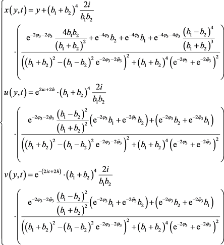
Parameter selection case two: Choosing $C_1=\frac{2b}{a}\cdot \left(a+bi\right)\cdot {\text{e}}^{2ic}$ , ${\tilde{C}}_1=\frac{2b}{a}\cdot \left(a-bi\right)\cdot {\text{e}}^{-2ic}$ , $C_2=\frac{2b}{a}\cdot \left(a-bi\right)\cdot {\text{e}}^{2ic}$ , ${\tilde{C}}_2=\frac{2b}{a}\cdot \left(a+bi\right)\cdot {\text{e}}^{-2ic}$ , then, we can get

$\{\begin{array}{l}x\left(y,t\right)=y-\frac{ab}{a^2+b^2}\left(\frac{b\sin 4{\phi }_1+a\sinh 4{\phi }_2}{a^2{\sinh }^{2}2{\phi }_2-b^2{\sin }^{2}2{\phi }_1}-\frac{2}{a}\right)\\ u\left(y,t\right)={\text{e}}^{2ic+2h}\cdot \frac{-2ab}{a^2+b^2}\left(\frac{a\sinh 2{\phi }_2\cos 2{\phi }_1+b\cosh 2{\phi }_2\sin 2{\phi }_1}{a^2{\sinh }^{2}2{\phi }_2-b^2{\sin }^{2}2{\phi }_1}\right)\\ v\left(y,t\right)={\text{e}}^{-\left(2ic+2h\right)}\cdot \frac{-2ab}{a^2+b^2}\left(\frac{a\sinh 2{\phi }_2\cos 2{\phi }_1+b\cosh 2{\phi }_2\sin 2{\phi }_1}{a^2{\sinh }^{2}2{\phi }_2-b^2{\sin }^{2}2{\phi }_1}\right)\end{array}$ (47)

2) Two pure image zeros

If choosing $k_1=i{b}_1$ , ${\tilde{k}}_1=-i{b}_1$ , $k_2=i{b}_2$ , ${\tilde{k}}_2=-i{b}_2$ , where $b_1>0$ , $b_2>0$ , and denoting ${\phi }_3=b_{1}y+\frac{t}{4b_1}$ , ${\tilde{\phi }}_3=b_{2}y+\frac{t}{4b_2}$ , then letting the parameter be $C_1=2i{b}_1{\text{e}}^{2ic}$ , ${\tilde{C}}_1=2i{b}_1{\text{e}}^{-2ic}$ , $C_2=2i{b}_2{\text{e}}^{2ic}$ , ${\tilde{C}}_2=2i{b}_2{\text{e}}^{-2ic}$ , we have

(48)

Remark 9: To our knowledge, the result (47) and result (48) are new.

4. Conclusion

In this article, we consider IVP for the 2SPE with initial value in Schwartz space. We begin with the Lax pair of 2SPE and then we formulate a Riemann-Hilbert problem in new coordinate (y, t), which implies that we can get the parametric form of soliton solutions in terms of the solution of the associated Riemann-Hilbert problem. After that, we can get the soliton solution by analyzing the residue condition of the Riemann-Hilbert problem. Last we obtain the soliton solutions, in particular the new breather-solution (47) and two soliton solution (48) were obtained.

Conflicts of Interest

The authors declare no conflicts of interest regarding the publication of this paper.

References

[1]	Schafer, T. and Wayne, C.E. (2004) Propagation of Ultra-Short Optical Pulses in Cubic Nonlinear Media. Physica D: Nonlinear Phenomena, 196, 90-105. https://doi.org/10.1016/j.physd.2004.04.007
[2]	Chung, Y., Jones, C.K.R.T., Schafer, T. and Wayne, C.E. (2004) Ultra-Short Pulses in Linear and Nonlinear Media. Nonlinearity, 18, 1351-1374. https://doi.org/10.1088/0951-7715/18/3/021
[3]	Matsuno, Y. (2011) A Novel Multi-Component Generalization of the Short Pulse Equation and Its Multisoliton Solutions. Journal of Mathematical Physics, 52, Article ID: 123702. https://doi.org/10.1063/1.3664904
[4]	Sakovich, A. and Sakovich, S. (2005) The Short Pulse Equation Is Integrable. Journal of the Physical Society of Japan, 74, 239-241. https://doi.org/10.1143/JPSJ.74.239
[5]	Brunelli, J.C. (2006) The Bi-Hamiltonian Structure of the Short Pulse Equation. Physics Letters A, 353, 475-478. https://doi.org/10.1016/j.physleta.2006.01.009
[6]	Sakovich, A. and Sakovich, S. (2006) Solitary Wave Solutions of the Short Pulse Equation. Journal of Physics A General Physics, 39, L361-L367.
[7]	Feng, B.F., Maruno, K.I. and Ohta, Y. (2010) Integrable Discretizations of the Short Pulse Equation. Journal of Physics A: Mathematical & Theoretical, 43, 555-557.
[8]	Brunelli, J.C. (2018) Super Extensions of the Short Pulse Equation. Communications in Nonlinear Science & Numerical Simulation, 63, 356-364. https://doi.org/10.1016/j.cnsns.2018.04.001
[9]	Xu, J. (2018) Long-Time Asymptotics for the Short Pulse Equation. Journal of Differential Equations, 265, 3494-3532. https://doi.org/10.1016/j.jde.2018.05.009