Classical and Relativistic Models for Time Duration of Gamma-Ray Bursts ()
1. Introduction
The theoretical efforts for gamma-ray bursts (GRBs) analyze: 1) the different predictions between cannonball and fireball model, see [1] [2] ; 2) the acceleration of ultrahigh-energy cosmic rays (UHECRs) at the afterglow phase, see [3] ; 3) a possible connection with high-energy neutrinos (HEN) and gravitational waves (GW), see [4] ; 4) the frames of hypersphere world-universe model (WUM), see [5] . We briefly recall that the time duration for gamma-ray burst (GRB) is measured without the knowledge of the redshift, see as an example [6] . The distance of GRBs is therefore unknown and the galactic or extra-galactic origin should be analyzed. We test therefore in the following the reliability of time duration for GRBs along two astrophysical hypothesis: 1) the GRBs are generated in external galaxies; 2) the GRBs are connected with the light curve (LC) of a supernova (SN). A first classification of time duration provides a division between short and long GRBs, with the boundary at » 2 s, see [7] . The form of the probability density function (PDF) which produces the better fit to the sequence of times is also subject of research, as an example, a two Gaussian-fits has been suggested by [8] and a lognormal PDF by [9] .
This paper reviews in Section 2 the current status of the observations for the time duration of GRBs. Section 3 develops a simple classic model for theoretical time duration for GRBs. Section 4 contains a simulation for time duration of GRBs based on the random generation of luminosity and distance luminosity. Section 5 derives a relativistic equation of motion for SN, deduces the relativistic flow of energy and finally evaluates the time duration for GRBS in a relativistic environment.
2. Preliminaries
This section reviews the observations of the Fermi Gamma-ray Burst Monitor (GBM) for the time duration and fits the data with the truncated lognormal PDF.
2.1. The Observations
Most of the typical GRBs have two stages: the initial prompt emission phase observed in the gamma-ray band and the following afterglow phase with multibands’ emission. The observational time duration is measured during the prompt emission phase with the typical energy band between tens of keV to hundreds of keV. Observationally, the light curve of the afterglow phase can be fitted by a broken power-law, but the light curve during the prompt emission phase is highly variable and completely different from the afterglow phase. The time duration of GRBs has been monitored by GBM in the 50 - 300 keV energy range, see the third catalog [6] which is available on line at http://cdsweb.u-strasbg.fr/. The above catalog reports two times of burst duration
and
which are defined as the interval between the times where the burst has reached 25% and 75% of its maximum fluence. Figure 1 reports the sky distribution of GRBs in Galactic coordinates.
A simple test on the isotropy of the arrival direction of GRBs can be performed dividing the the surface area of a sphere of unit radius in
boxes of equal area. We then choose N in order to have » 7 theoretical events,
, assuming a uniform distribution on the total surface area, which means
. We now evaluate the observed averaged number of GRBs in each box, n, which turns out to be
. The goodness of the isotropy is evaluated through the percentage error,
, which is
(1)
![]()
Figure 1. Sky distribution of GRBs in Galactic coordinates projected using the Mollweide projection.
The low value of the percentage error for the isotropy allows to state that:
• the GRBs have an extra-galactic origin;
• the spatial distribution of GRBs is isotropic.
The histogram of time distribution for GRBs for the case of
in Figure 2 and in Figure 3 for the case of
.
Scheme 1 and Scheme 2 report the main statistical parameters of
and
respectively.
2.2. The Fit
The high number of decades, » 4, covered by the distribution of
and
suggests to fit the data with the truncated lognormal (TL) PDF
(2)
where x is the random variable,
is the lower bound,
is the upper bound, m is the scale parameter and
is the shape parameter, see [10] for more details. Scheme 3 and Scheme 4 report the four parameters of the TL for
and
respectively. Scheme 4 reports also the parameters of the lognormal PDF as well the maximum distance,
, between the theoretical and the observed distribution function (DF) in the Kolmogorov-Smirnov test (K-S), see [11] [12] [13] .
The DF is
(3)
![]()
Figure 2. Frequencies distribution (linear scale)) of
(decimal logarithm scale) for GRBs.
![]()
Figure 3. Frequencies distribution (linear scale)) of
(decimal logarithm scale) for GRBs.
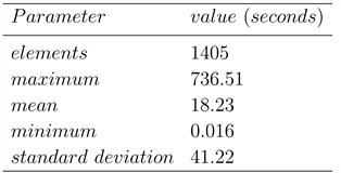
Scheme 1. The sample parameters of
for GRBs in seconds.
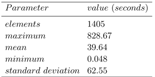
Scheme 2. The sample parameters of
for GRBs in seconds.

Scheme 3. The TL parameters of
for GRBs.
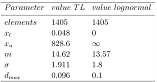
Scheme 4. The TL PDF and lognormal PDF parameters of
for GRB.
A random generation of the variate X can be found by solving the following non linear equation
(4)
where R is the unit rectangular variate.
3. A Classical Model for the Light Curve
We assume that the observed radius-time relationship,
, for SN has a power law dependence of the type
(5)
where
is a constant and
a parameter which can be fixed by the observation of the temporal evolution of the radius of a SN, in the case of SN 1993J
, see [14] . At time
the radius
is
(6)
The velocity,
, is
(7)
and the velocity at time
is
(8)
In classical physics the density of kinetic energy, K, is
(9)
where
is the density and
the velocity. In presence of an area
and when the velocity is perpendicular to that area, the mechanical flux of kinetic energy
is
(10)
which in SI is measured in W and in CGS in erg s−1 see Formula (A28) in [15] . In our case,
, which means
(11)
The density in the advancing layer as function of the radius,
, is assumed to scale as
(12)
where
is the density at radius
. According to previous formula, the scaling law for the mechanical luminosity as function of the time is
(13)
where
is the mechanical luminosity at
. The observed luminosity at a given frequency
,
, is assumed to be proportional to the mechanical luminosity
(14)
where
is a constant of conversion. The luminosity at a given range of energy is expressed in erg/s in CGS and W in SI. As a useful example the astrophysical version of the luminosity at
is
(15)
where
is the radius at
in pc,
is the velocity at
in km/s,
is the light velocity in km/s and
is the number density expressed in particles cm−3 (density
, where
).
The observed flux,
, as a function of the luminosity distance,
, is
(16)
or
(17)
where
. The observed flux at a given range of energy is expressed in erg/scm2 in CGS and W/m2 in SI. An on line collection of light curves for GRBs is made by the Swift GRB Mission and can be found at http://swift.gsfc.nasa.gov/index.html, see also [16] [17] : the band of the
observations is (0.3 - 10) kev. As a practical example we processed GRB161214B, see [18] , with review data in Scheme 5, and real data available at http://www.swift.ac.uk/xrt_curves/00726885/. Figure 4 displays the LC of such burst as well a power law fit.
![]()
Figure 4. Light curve of GRB161214B in the first 100 seconds (empty stars) and power law fit (dotted line).

Scheme 5. Some parameters of GRB161214B.
A first numerical analysis of the observed flux,
, versus time relationship can be done by assuming a power law dependence
(18)
where the two parameters
and
are found from a numerical analysis of the data, see Scheme 5. We now match the observed value of
with the theoretical exponent given by Equation (17)
(19)
The above equation allows to deduce
once
and
are given: as an example, when
and
,
. The decreasing flux will be visible until a minimum value of threshold in the flux
is reached. As an example the instrument Windowed Timing (WT) of X-ray telescope (XRT) on the Swift satellite has a threshold value of
. Therefore the GRB will be visible up to a maximum value in time of
(20)
or
(21)
where
is the observed flux at
.
4. The Simulation
A simulation of the duration time for GRBs according to Equation (20) requires the ratio of two two lognormal PDFs (one for
and the other one for
) and a cosmological environment.
4.1. The Ratio of Two Lognormal PDFs
We now evaluate the mean and the variance of the ratio of two lognormal
distributions,
. From the fact that
and
and
are lognormally distributed, it turns out that
and
are distributed as a normal PDF. We assume that
and
have means
and
, variances
and
, and covariance
(equal to zero if X and Y are independent) and are jointly normally distributed. The difference
is then distributed as a normal PDF with mean
and variance
.
Note that
, which means that
is distributed as a lognormal
PDF with parameters
and
.
4.2. Cosmological Models
We deal with two cosmologies: the LCDM cosmology and the plasma cosmology. The the LCDM cosmology is characterized by three parameters which are the Hubble constant,
, expressed in kms−1Mpc−1 and the two numbers
and
,, see Scheme 6.
A simple expression for the luminosity distance,
, in LCDM is obtained with the minimax approximation (
)
(22)
More details on the analytical derivation of the luminosity distance in terms of Padé approximant can be found in [19] .
The plasma cosmology is characterized by one parameter which is
and by a simple formula for the luminosity distance which is the same of the distance,
,
(23)
see [20] [21] [22] [23] and see Scheme 6.
A careful examination of Equation (20) which gives the time duration for a GRB isolates five fixed basic parameters which are
,
,
,
,
and two random parameters are ,
,
. In order to allow the simulation the five fixed parameters are reported in Scheme 7.
The variable
is generated in a random way which follows a TL PDF with the following meanings:
lower luminosity,
upper luminosity and
the scale, see Scheme 8.
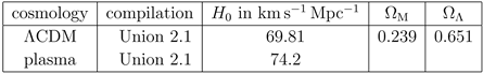
Scheme 6. Numerical values for parameters of the two cosmologies.
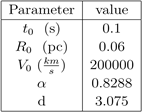
Scheme 7. The fixed parameters of the simple model.
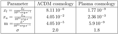
Scheme 8. The parameters of the simulation for L in LCDM and plasma cosmology.
The theoretical luminosity at
,
, is obtained inserting in Equation (15) the number density
for which
.
The variable
, in the case of LCDM or plasma cosmology, is generated in a random way which follows a TL PDF with the following meanings:
lower luminosity distance,
upper luminosity distance and m the scale , see Scheme 9.
Once a sequence of theoretical times of duration is obtained according to Equation (20), see results in Scheme 10, we compare the observed and simulated data, see Figure 5 and Figure 6.
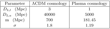
Scheme 9. The parameters of the simulation for
in LCDM and plasma cosmology.
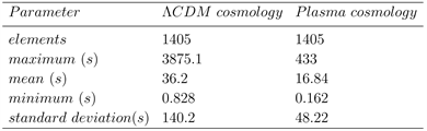
Scheme 10. Theoretical time duration for GRBs in seconds.
![]()
Figure 5. Frequencies distribution (linear scale)) of
(decimal logarithm scale) for GRBs (full line) and theoretical simulation in the case of the LCDM cosmology (dotted line) with parameters as in Scheme 8 and Scheme 9.
![]()
Figure 6. Frequencies distribution (linear scale) of
(decimal logarithm scale) for GRBs (full line) and theoretical simulation in the case of the plasma cosmology (dotted line) with parameters as in Scheme 8 and Scheme 9.
The theoretical reason which allows to fit the ratio of two lognormal PDFs with another lognormal is outlined in Section 4.1.
5. Relativistic Case
The density,
, of the ISM at a distance r from the SN is here modeled by a Plummer-like profile, see [24] ,
(24)
where r is the distance from the center,
is the density,
is the density at the center,
is the distance before which the density is nearly constant, and
is the power law exponent at large values of r. The following transformation,
, gives
(25)
The total mass
comprised between 0 and r, when
, is
(26)
The relativistic conservation of momentum, see [25] [26] [27] , states that
(27)
with
(28)
and
(29)
where
is the initial radius of the advancing sphere,
is the initial velocity at
and
is the light velocity.
The relativistic conservation of momentum for a Plummer profile with
is
(30)
(31)
(32)
(33)
(34)
The relativistic transfer of energy through a surface,
, is
(35)
where p is the pressure here assumed to be
; see Equation (A31) in [15] or Equation (43) and Equation (44) in [28] .
The astrophysical version of the relativistic transfer of energy (the luminosity) at
is
(36)
where
is the radius at
in pc.
In the case of a spherical cold expansion
(37)
We now assume the following power law behavior for the density in the advancing thin layer
(38)
and we obtain
(39)
We can now derive
in two ways: 1) from a numerical evaluation of r(t) and v(t); 2) from a Taylor series of
of the type
(40)
The first two coefficients are
where
(41)
and
(42)
Figure 7 compares the numerical solution for the luminosity and the series expansion for the luminosity about the ordinary point
.
The relativistic theory is now applied to GRB050814 at 0.3 - 10 kev in the time interval 10−5 - 3 days, see [29] , with data available at http://www.swift.ac.uk/xrt_curves/150314 .
The theoretical flux without absorption is given by Equation (16) and Figure 8 reports the comparison of the theoretical flux and the observed one.
The presence of the absorption can be modeled as
(43)
![]()
Figure 7. Numerical
computed according to Equation (35) (dotted line) and series solution of order 7 as given by Equation (36) (full line). Data as in Scheme 11.
![]()
Figure 8. The XRT flux of GRB050814 at 0.3 - 10 kev (empty stars) and theoretical curve as given by the relativistic numerical model, see Equation (35), in presence of absorption as given by Equation (39) (full line).
where
is the optical thickness here assumed to be dependent from the time. As a model for
as function of time we select a logarithmic polynomial approximation, of degree 5 , see [30] for more details. Figure 9 reports the LC for the relativistic case with absorption for GRB 050814.
The Relativistic Simulation for Time Duration
In the relativistic case the theoretical luminosity is provided by a series solution of order 7, see Equation (36), The fixed parameters adopted for the simulation of duration time are reported in Scheme 12.
The random luminosity L is generated according to a TL PDF, see Scheme 13.
The value of
which allows to generate
in a random way is deduced by
with L as evaluated in Equation (32). The distance luminosity,
, in the case of LCDM or plasma cosmology, i randomly generated according to a TL PDF, see Scheme 14.
The sequence of theoretical times of duration is obtained in a numerical way, see results in Scheme 15. The observed and simulated data are displayed in Figure 10 and Figure 11.
![]()
Scheme 11. Numerical values of the parameters used in the Plummer relativistic solution.
![]()
Scheme 12. Numerical values of the parameters used in the Plummer relativistic simulation for duration time of GRBs.
![]()
Scheme 13. The parameters of the relativistic simulation for L in LCDM and plasma cosmology.
![]()
Scheme 14. The parameters of the relativistic simulation for DL in LCDM and plasma cosmology.
![]()
Scheme 15. Theoretical time duration for GRBs in seconds in a relativistic framework.
![]()
Figure 9. Frequencies distribution (linear scale)) of
(decimal logarithm scale) for GRBs (full line) and theoretical simulation in the case of the LCDM cosmology (dotted line) with parameters as in Scheme 8 and Scheme 9. The model is relativistic, see Equation (35) (full line) without absorption.
![]()
Figure 10. Frequencies distribution (linear scale)) of
(decimal logarithm scale) for GRBs (full line) and theoretical simulation in the case of the plasma cosmology (dotted line) in a relativistic framework with parameters as in Scheme 13 and Scheme 14.
6. Conclusions
Extra-galactic versus Galactic origin
The direction of arrival of GRBs shows an isotropic universe with a percentage error of 2.4%. This means that the GRBs are originated in external galaxies in a random way as suggested by [31] .
Truncated lognormal distribution
The lognormal PDF is usually adopted to model the duration time of GRBs, see [9] . The TL PDF improves the reliability of the fit, see Scheme 2. Careful attention should be paid to the fact that a two-Gaussian and a three-Gaussian fit are also used to model the duration times for GRBs, see [8] .
A simple model
The theoretical time of duration can be derived from the light curve for GRBs. A power law approximation for the time of expansion of a shell, see Equation (5), coupled with a power law behavior for the density as function of the radius, see Equation (12), allows to derive a formula for the theoretical luminosity, see Equation (14). A theoretical time of duration is obtained, see Equation (20) which contains an evaluation of the luminosity and the luminosity distance. The cosmological evaluation of the luminosity distance is given both in LCDM cosmology and plasma cosmology. The results are given in Scheme 10, Figure 5 and Figure 6.
Relativistic model
The temporal evolution of a SN in a medium of the Plummer type,
, can be found by applying the conservation of relativistic momentum in the thin layer approximation. This relativistic invariant is evaluated as a differential
![]()
Figure 11. Frequencies distribution (linear scale)) of
(decimal logarithm scale) for GRBs (full line) and theoretical simulation in the case of the plasma cosmology (dotted line) in a relativistic framework with parameters as in Scheme 13 and Scheme 14.
equation of the first order, see Equation (26). Two different relativistic solutions for the theoretical luminosity as a function of time are derived: 1) a numerical solution, see Equation (35); 2) a series solution, see Equation (36), which has a limited range of validity,
.
The coupling of the previous series with a logarithmic polynomial approximation allows to model fine details such as the oscillation in LC visible at »1000 s in GRB161214B , see Figure 8.
The relativistic time of duration is reported in in Scheme 15, Figure 9 and Figure 10.
An enlightening example of such relativistic simulation is absence of bursts at
visible in Figure 9. This means that the claimed boundary at
which divides the short by the long bursts, see [7] , is due to random events rather than two different kind of bursts.
Acknowledgements
This work made use of data supplied by the UK Swift Science Data Centre at the University of Leicester.