On the Kinetic Energy of the Projection Curve for the 1-Parameter Closed Spatial Homothetic Motion ()
1. Introduction
Kinetic energy is the energy that an object possesses because of its motion. The kinetic energy of the object having a linear orbit is called displacement kinetic energy, object with circular orbit called the rotational kinetic energy and also the kinetic energy of the object having high speed called relative kinetic energy.
Kinematics is a branch of mechanics dealing with the reasons that cause the motion to be ignored and how the movement occurs. For this reason, kinematics is generally called as the motion geometry. In kinematics, motion is called open or closed motion, depending on whether the trajectory curves are open or closed. There are many studies on the account of the fields of the trajectory curves. As an example, the Steiner area formula and Holditch theorem can be given [1] [2] . The results obtained in these studies have attracted the attention of many mathematicians and have been a source of inspiration for many studies. Accordingly, H. R. Müller generalized the relationship between the polar moment of inertia and the calculation of the trajectory field [3] . Tutar and Kuruoğlu expressed the Stiener area formula of closed curves for 1-parameterized planar homothetic motion [4] . Düldül generalized the Holditch theorem for closed space curves [5] . Düldül and Kuruoğlu had calculated the polar moment of inertia for the Holditch type theorem of complex plane trajectory curves during 1-parameter closed homothetic motion [6] . Düldül calculated polar moment of inertia of the projection curve at any point under 1-parameter homothetic motion, then calculated the volume of these points under the 3-parameter homothetic motion. Thus, using the polar moment of inertia and volume formula, similar results to the spatial Holditch-type theorem were obtained [7] . Inan studied the Steiner area formula and polar moment of inertia for closed trajectory curve under homothetic motion in planar kinematics [8] . In addition, the kinetic energy formula for 1-parameter closed planar homothetic and inverse homothetic motion are taken by Tutar and İnan [9] [10] . On the other hand, Dathe and Gezzi calculated the Steiner area formula and the polar moment of inertia for the motion composed of fixed and moving systems between the knee and hip joints during human walking and correlated the polar moment of inertia with the Stiener area formula [11] [12] .
In this study, the kinetic energy of the projection curve under 1-parameter closed homothetic space motion is investigated and some results are obtained.
2. Kinetic Energy of the Projection Curve
Let
and
be moving and fixed planes,
and
be origin of their coordinate systems and also
direct motion with t parameter between these systems. By taking displacement vector
, total rotation angle
,
is called the trajectory of the fixed point
, according the moving system. In that equation, h is a homothetic scale of the motion
. Rotation matrix
, vector
and displacement vector
are the continuous differentiable function of the a reel parameter t.
Motion with a first order in the time derivate can be given
which is the integral over the kinetic energy of point with mass
.
Let X be a fixed point at moving space and coordinates of the X according to
system be
, and
can be written.
If the displacement vector is expressed by
the position vector of the fixed point x, on the 1-parameter closed homothetic spatial motion can be written as following:
(2.1)
Fixed point
draws a closed curve while motion. The projection of that closed curve on the plane P, in the direction of the unit
vector, is also closed curve (Image 1).
Let show this closed curve with (
) and projection of the point X on the plane be with
. And also plane M and origin of the fixed plane coincide. From Image 1, it can be written:
or
(2.2)
By using Equation (2.2),
(2.3)
If the Equation (2.3) is derivated, we obtain
(2.4)
And if the norm of the Equation (2.4) is determinated, we get
(2.5)
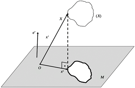
Image 1. The projection of that closed curve on the plane P.
Kinetic energy of the closed projection curve (
) according to origin point
is
(2.6)
Integration boundary of Equation (2.6) is between 0 and T. If Equation (2.5) is replaced in Equation (2.6) and taking into account Equation (2.1), we obtain,
(2.7)
By using Equation (2.7), kinetic energy of the origin point of the projective curve on the plane M is
(2.8)
If
are taken, we get
(2.9)
and also
(2.10)
If the Equation (2.8), Equation (2.9) and Equation (2.10) are replaced in Equation (2.7), we obtain,
(2.11)
At Equation (2.11),
By using these assumptions the kinetic energy formula of the fixed
of the closed projective trajectory curve on the plane M is
(2.12)
Equation (2.12) is a quadratic equation according to
components. As a result of Equation (2.12), the following theorem can be given.
Theorem 1:
The projection of all fixed points of moving space E, which have the equal kinetic energy, are located on the same sphere.
Let take into consideration
where
is a continuous function. According to the mean value theorem of integral-calculus, there exists at least a point
such that the following equation holds:
(2.13)
If the moving coordinate system are chosen to be
for
and by using to the mean value theorem of integral-calculus to the
there exists at least a point
such that the following equation holds
(2.14)
In that case, by using Equation (2.12)
(2.15)
is obtained. Additionally, since
for
;
can be written. Furthermore, if the both side of the Equation (2.12) multiply with
and integrate, we get
Since
,
or
(2.16)
can be written. Let, L be the maximal value of the
function at
. In that case, for
,
and
can be written. Since
, we get
By using Equation (2.16),
can be written. Because of the
is continuous at
, there exists at least a point
such that the following equation holds
Thus,
(2.17)
can be written. Since
, we have
If these equations are arranged,
can be written. There exists
such that the following equations hold,
or
(2.18)
In this case, we have
And by using Equation (2.17)
(2.19)
can be written. If Equation (2.19) is replaced in Equation (2.15), kinetic energy formula of the projection curve of fixed point, which is chosen from moving space, under the 1-parameter closed spatial motion can be written as:
(2.20)