An Approach to Fault Diagnosis of Rotating Machinery Using the Second-Order Statistical Features of Thermal Images and Simplified Fuzzy ARTMAP ()
1. Introduction
Together with the development of science and technology, modern rotating machinery in industry has been increasingly developing toward large scale, high speed operation, more precision, and high degree of automation. In the meantime, its structure is gradually becoming more complex, increasing the degree of integration where the entire production could be interrupted once a part or a link fails. These demand to improve the capability of condition monitoring and fault diagnostic technologies and use effective signals so that the potential faults of such machine can be early detected and diagnosed. Traditionally, acoustic and vibration signals are widely used for machine condition monitoring and fault diagnosis due to their easy-to-measure characteristics and their useful information of machine state containing in the features for analysis. Some outstanding works referred in [1] - [6] have been successfully used these signals for machine fault detection and fault diagnosis.
However, it is challenging to extract useful features for acoustics and vibration due to noise contaminating in the acquired signals. Indeed, the most obvious technique to obtain a vibration signal is by direct measurement using vibration transducer rigidly mounted on machine. This not only requires a high-perfor- mance vibration transducer which is capable of withstanding harsh environmental condition, but also demands a costly investment for measuring instrument where a large number of measuring points are concerned [7] . A main disadvantage is that the vibration signals contain strong noise which needs an effective signal processing tool to get useful information. Similarly, the acoustic signal is easily contaminated in a normal industrial environment due to the fact that airborne sound from machine is noisy and complex. That is a reason why the acoustic signal has been received slight attention for machinery condition monitoring and fault diagnosis [8] . It could state that alternative signals being more accurate are necessary.
Generally, in order to deal with rotating machinery fault diagnosis based on intelligent techniques, the features presenting the characteristics of signal are first extracted. It is similar to the approaches of using thermograms where their extracted features maybe roughly divided into three categories: structural, spectral, and statistical. In structural approaches, texture primitive, the basic element of texture, is used to form a more complex texture pattern by grammar rules that specify the generation of texture pattern [15] . The advantage of the structural approach is that it provides a good symbolic description of the image; however, this feature is more useful for synthesis than analysis tasks [16] . In spectral approaches, the texture image is transformed into frequency domain, and then the extraction of texture features can be carried out by analyzing the power spectrum. The spectral approaches are limited in practice due to lack of either spatial localization or filter resolution at which one can localize a spatial structure in natural textures. Finally, statistical approaches do not attempt to understand explicitly the hierarchical structure of the texture. Instead, they represent the texture indirectly by the non-deterministic properties that govern the distributions and relationships between the grey-levels of an image. This is the reason why statistical texture features are commonly used in machine fault diagnosis.
So far, most of studies of fault diagnosis using thermogram have only focused on the histogram features, which are the first-order statistical texture features, due to their simplicity. The histogram features only provide information related to the grey-level distribution and ignore the spatial interaction among image pixels. They are not able to measure if all low-value grey-levels are positioned together, or they are interchanged with the high-value grey-levels [17] . It was early argued that they were insufficient for adequate texture description and second-order statistical features were required, as efficiently reflected in features computed from the co-occurrence matrix [18] . Furthermore, approaches based on the second-order statistics have achieved higher discrimination rates than the spectral and structural approaches have [19] . Consequently, the second-order statistical features are considered for fault diagnosis in this paper and extracted from the gray-level co-occurrence matrix (GLCM), which was firstly introduced by Haralick et al. [18] . In addition, other features including cluster shade, cluster prominence, and maximum probability proposed in [20] [21] [22] are also investigated.
Based on the features, the machine conditions could be precisely identified through classification models. These classification models have a wide range of approaches which are varied from model-based to artificial intelligence-based. Among these, artificial intelligence (AI) is regularly used owing to their accuracy and flexibility. Such AI models require “minimum configuration intelligence” since no detailed analysis of the fault mechanism is necessary, nor is any modeling of the system required. Once an AI model is used, fault classification can be accomplished without a highly trained and skilled personnel required. A review of techniques including AI for machinery fault diagnosis could be found in the study of Jardine et al. [23] . Recently, SVM [24] belonging to statistical approaches has been considered as a remarkable model in classification and attracted much attention by researchers in fault diagnosis. However, in our previous work [25] , the comparative performance of SVM and simplified fuzzy ARTMAP (SFAM) [26] was carried out and the result shows that SFAM is superior to SVM in aspect of the accuracy and computational cost. Accordingly, SFAM is used as the classification to diagnose the conditions of rotating machinery in this study. Furthermore, its classification results and those of other traditional AIs such as back-propagation NN and probabilistic NN are carried out to appraise the advantages of the proposed framework.
2. Theoretical Background
2.1. GLCM and Second-Order Statistical Texture Features
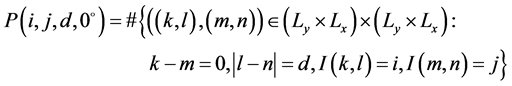
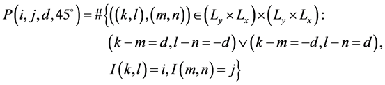
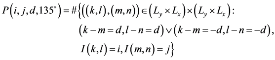
GLCM is a matrix of the relative frequencies Pij of two neighboring pixels having grey-level i and j. This matrix is a function of two parameters: relative distance measured in pixel numbers d and their relative orientation θ being quantized to 45˚ intervals. Thus, for different values of θ and d, different GLCMs are generated. Due to the intensive nature of computations involved, only the distance d = 1 or 2 pixels with angles θ = 0˚, 45˚, 90˚, and 135˚ are normally considered [18] . Suppose an image to be analyzed in rectangle and has Nx columns and Ny rows. Suppose that the grey-level appearing at each pixel is quantified to Ng levels. Let  be the columns,
  be the rows, and
 be the set of Ng quantized grey-levels. The set
  is the set of pixels of the image ordered by their row-column designations. The image I can be represented as a function that assigns some grey-level in G to each pixel or pair of coordinates in
 ;
; . The unnormalized frequencies can be defined by
 (1)
(1)
 (2)
(2)
 (3)
(3)
 (4)
(4)
where # denotes the number of elements in the set.
Using the co-occurrence matrix above, the second-order statistical features are given in Table 1.
2.2. The mRMR Based Feature Selection
Mutual information (MI) is a quantity that measures the level of similarity between features and the level of correlation between feature and class. Accordingly, the MI of features should be minimized to decrease the redundancy among them and MI of feature and class should be maximized to retain the high relevance. mRMR [27] is a MI based feature selection method simultaneously considering both the relevance and the redundancy in a framework. In term of MI, the relevance of a feature set S for the class c is defined by the mean value of all MI values between the individual feature fi and the class c. The criterion of maximum relevance is given as follow:
 (5)
(5)
The redundancy of all features in the set S is the mean value of all MI values between the feature fi and fj. The minimum redundancy criterion is defined as:
 (6)
(6)
The mRMR feature set is obtained by optimizing the conditions described in Equations (5) and (6) simultaneously. In order to optimize these conditions, it is necessary to combine them into a single criterion function. According to [28] , the two simplest combinations of these conditions are mutual information difference (MID) and mutual information quotient (MIQ) forms:
 (7)
(7)
 (8)
(8)
mRMR uses the following algorithm to solve this optimization problem. The first feature is selected according to Equation (5), i.e. the feature with the highest . The remaining features are selected in an incremental way: earlier selected features remain in the feature set. Suppose that m features are already selected
![]()
Table 1. The second-order statistical features.
for the set S, we want to select additional features from the set . We optimize the MI between both features and class label based on the following two conditions:
 (9)
(9)
![]() (10)
(10)
The condition in Equation (9) is equivalent to the maximum relevance condition in Equation (5), while Equation (10) is an approximation of the minimum redundancy condition of Equation (6). The two ways to combine relevance and redundancy described in Equations (7) and (8) lead to the selection criteria of a new feature:
![]() (11)
(11)
![]() (12)
(12)
2.3. Simplified Fuzzy ARTMAP Network (SFAM)
SFAM is a simplified version of fuzzy ARTMAP [29] by reducing the complicated and redundancy architectures that is the main drawback of the original model for classification task. As a result, SFAM is faster than fuzzy ARTMAP and easier to understand. The details of this network could be found in [26] .
3. The Proposed Framework
The proposed framework for machinery fault diagnosis is shown in Figure 1. This framework is initiated by the capture of thermal images of different machine conditions; then, these images are preprocessed for cropping the regions of interest (ROIs), removing the noise, and enhancing the contrast in ROI using the histogram equalization (HE) algorithm. For further improving the image information to increase the diagnosis accuracy, these images are enhanced by using a combined method of bi-dimensional empirical mode decomposition and PCA fusion (BEMD-PCAF) proposed in our previous study. Further details of this method could be found in [30] . After being enhanced, second-order statistical features are extracted from the GLCMs. Nevertheless, the feature set contains
![]()
Figure 1. Proposed framework for machinery fault diagnosis.
many redundant as well as relevant features leading to the necessity of feature selection to reduce the computation cost, select prominent features, and eliminate the irrelevant features for avoiding the issue of dimensionality curse. Generally speaking, feature selection methods can broadly fall into three families: filter-based, wrapper-based and embedded methods [31] . Among these, filter-based method is widely used due to its computational efficiency and is employed in this study via mRMR. Finally, the selected feature set is partitioned into training set and test set to build the classifier and validate it, respectively.
4. Experiment
To validate the proposed framework, a series of experiments were carried out by using a fault simulator which consists of driving motor, shaft, disk, PC for saving data, and thermal camera as shown in Figure 2. The short shaft, which is of 30 mm diameter and is supported by two ball bearings at the ends, was attached to the shaft of the driving motor through a flexible coupling. This coupling is also used to adjust the misalignment condition on the fault simulator. In order to create the unbalance condition, a disk with many available tapped holes to add extra mass was attached on the shaft. The variable speed DC motor (0.5 HP) with speed up to 3450 rpm was used as the driving motor.
The thermal camera, which is the key device for image acquisition, used for experiments was a long-wave infrared camera from FLIR with the thermal sensitivity of 0.08˚C at 30˚C. Some its parameters require to be set consisting of emissivity (0.9), relative humidity (50%), and distance between the focal length of camera and object (2 m). All of these parameters are chosen according to experimental condition and they were maintained constant in the experiments. The main specifications of the thermal camera and fault simulator are shown in Table 2. The experimental procedure for each condition was carried out as following: the speed of the motor was increased gradually up to 900 rpm and was held for five minutes to enable the machine to reach its stable condition. The image acquisition processes for normal, misalignment, mass unbalance, and bearing
fault conditions were then conducted. These faults were created by adjusting the dial screws on the left and right ends of the base plate of the simulator (misalignment), adding a screw 0.02 kg in one of the tapped holes in the rotor disk (mass unbalance), and using outer-race faulty bearing with the defect size 0.3556 mm. For each condition, twenty samples (20) were taken and saved directly to the PC.
5. Results and Discussion
5.1. Image Preprocessing and Feature Calculation
The experimental images collected from different conditions of rotating machinery contain many regions of the fault simulator and background. To focus on fault diagnosis of rotating machinery and avoid unnecessary computation for other regions, a rectangle ROI with the size of 150 × 20 pixels is designated as shown in Figure 3. Then, HE technique is employed for the ROI to augment the
![]()
Table 2. Main specification of thermal camera and fault simulator.
contrast. For further improving the image information to increase the diagnosis accuracy, these images are enhanced by BEMD-PCAF. The result of these preprocessing showed in Figure 4 indicates that the visibility of the original image has been improved.
Next, the process of feature calculation is carried out to extract the second- order statistical features introduced in section 2.1. As mentioned, these features are computed from each of the GLCMs obtained by using different values of the relative distance d and the relative orientation θ. The distance d parameter is of importance in the computation of GLCM. As reported in the studies [18] [22] , the classification result was best when using features from matrices of d = 1 or 2. Hence, the relative distance d as 1 with the orientation θ of 0˚, 45˚, 90˚, and 135˚ is implemented for this study, then averaging these values. In addition, six different values of grey-levels Ng = 8, 16, 32, 64, 128, 256 are also investigated to appraise which value can provide the highest accuracy. Theoretically, 38 features consisting of 19 features mentioned in section 2.1 and their ranges are computed from the image for each grey-level value. However, the feature f14, namely maximal correlation coefficient, is not used in this study due to the fact that some values of px(i) or py(j) are equal of zeros leading to computational instability. The visualization of the feature distribution in the feature space is shown in Figure 5, where the features of maximum probability, cluster shade, and cluster prominence are presented. It can be seen that the features of image after using BEMD-PCAF are better in cluster of the features being in same condition and superior to separation between the features of different condition than the ones enhancing by HE. This helps the classification more easily attaining the high accuracy without necessity of using any methods to map the features into another space.
5.2. Feature Selection and Classification
The number of features obtained from the previous stage is high dimensionality. Too many features may unnecessarily increase the complexity of the training and classification task; conversely, insufficient selection of features may have a detrimental effect on the classification results. In feature-based techniques, there are two tactics to reduce the high dimensionality as well as select the salient features which are high correlation with the target class label: feature selection and feature extraction. Feature extraction is a technique that transforms the existing features into a lower dimensional space, while feature selection selects a subset of the existing features that optimizes one or more criteria. Notice that the transformation of feature extraction may provide a better discrimination but cannot
![]()
![]() (a) (b)
(a) (b)
Figure 4. (a) Original image, (b) Enhanced image.
![]() (a)
(a)![]() (b)
(b)
Figure 5. Second-order features of image with grey-level = 8: (a) Enhanced by HE, (b) Enhanced by BEMD-PCAF.
retain the original physical interpretation as feature selection.
In this study, the feature selection method based on mRMR algorithm using MID criterion is used for the purpose of the dimensionality reduction due to its stability in producing feature subsets even MID and MIQ can provide a similar accuracy [32] . Since mRMR is a filter-based method, its subset features necessitate combining with classifier to evaluate the diagnosis accuracy. For each grey-level value, the total features which have 80 samples for 4 machine conditions are randomly partitioned by holdout validation method into 50% for training set to generate the SFAM diagnostic model and the rest for test set to evaluate the model’s accuracy. In the training mode, SFAM is trained by basic network setting, i.e. fast learning β = 1 and conservative mode α = 0.001. The value of vigilance parameter (VP) varies from 0 to 0.9 with an increment step of 0.1 to investigate the performance. Due to the randomized selection of samples for the training set and test set, the process of partitioning total features and classes, selecting feature, training and evaluating diagnostic model is repeated 10 times and then average the classification results. In the feature selection process, the number of the selected features is gradually increased from 1 to 36 to determine the number of features sufficing for classifier.
The classification results of SFAM in the testing mode with different values of VPs, grey-levels, and the number of selected features obtained from mRMR are shown in Figure 6. It can be seen that most of the classification accuracy achieve 100% with only one feature selected when the grey-level of 32. This indicates that the selected feature, namely cluster shade in this case, gives a highest relevance with the target labels. However, this accuracy is reduced when increasing the number of selected features over 4. The second grey-level where SFAM classifier can provide a high accuracy and stable for all VP values is of 128; however, the classifier only reaches to 100% accuracy after 3 features selected which are respectively mean of sum average, mean of variance, and cluster prominence. For the other grey-levels, SFAM either achieves lower accuracy, for instance grey-level of 8 and 256, or uses a large number of features to attain a significant accuracy such as grey-level of 64. With the grey-level of 8, SFAM only achieves 99.64% once the selected features are 26 for the value of VP as 0, or achieves 100% when the number of features of 27 for VP of 0.8, which are high computational cost; for other values of VP, SFAM provides a lower accuracy. It is similar for the grey-level of 256. In case of grey-level of 64 where SFAM provides better results, the classification accuracy can attain 100% when the selected features is of 4; however, this only happens in some of VP values such as 0, 0.4, 0.6, 0.7, and 0.8. Thus, the grey-levels of 32 and 128 can give good performance of classification and are chosen for the comparative study in the next section.
5.3. Comparative Performance of SFAM, BPNN, and PNN
As observed in Figure 6, with the VP value of 0.4, SFAM can give a high and stable performance for both grey-levels of 32 and 128. Four selected features used for SFAM in these cases are also applied for back-propagation neural networks (BPNNs) and probabilistic neural networks (PNNs) to evaluate the three-classifier performance. In case of grey-level of 32, the selected features obtained from mRMR are cluster shade, mean of contrast, dissimilarity, and mean of difference variance. In case of grey-level of 128, mean of sum average, mean of variance, cluster prominence, and mean of maximum probability are selected. The networks are trained with ten hidden nodes and Levenberg-Marquardt algorithm. The classification results of the three classifiers are shown in Table 3. It can be seen that SFAM and PNN are superior to BPNN in case of the grey-level of 32. In case of grey-level of 128, BPNN accuracy is higher than ones of SFAM and PNN when one number of selected features is used, and vice versa. Table 3 also shows the training time of the classifiers when one feature is used
![]()
Figure 6. Classification results of SFAM.
for classification. The training time of SFAM is significantly low in comparison with ones of BPNN and PNN. This indicates that SFAM can give better performance with low computational cost that is very useful for real application where huge data could be used.
![]()
Table 3. Classification accuracy of SFAM, BPNN, and PNN.
6. Conclusion
This paper has presented a new approach of the second-order statistical features of thermal image for fault diagnosis by introducing them into the framework including mRMR and SFAM. The experimental thermal images of a simulator with different conditions such as normal, misalignment, faulty bearing, and mass unbalance are used for this investigation. The second-order statistical features are extracted from these images with the grey-levels of 8, 16, 32, 64, 128, and 256. Then, mRMR based on MID is employed to select the features which have high relevance to the machine condition to input the SFAM classifier. As a result, the classification accuracy of SFAM achieves 100% with only cluster shade feature selected from whole the feature set when the grey-level of 32 is used. In another grey-level of 128, SFAM can reach to 100% accuracy until 3 features are selected. Additionally, a comparative study of the performance of SFAM and other traditional networks BPNN and PNN has been carried out. The results show that SFAM not only provides a better performance but also has insignificantly computational cost. This indicated that SFAM is eminently suitable to use for real fault diagnosis applications.