On the Quantum Entanglement Reinterpretation Using the Time as Real Instantaneous Signal Field

Elsadig Naseraddeen

Founder and General Manager, Information Fluxes-FZE, Dubai, UAE.

DOI: 10.4236/jmp.2017.86054                

Abstract

In relativistic mechanics the time-like vector characterize the motion in spacetime with speed faster than the speed of light in vacuum c in which the line element ds²=c²dt²-dx²-dx²-dz² is less than zero (where is infinitesimal change in time, and are infinitesimal change in space), thus the time in relativistic mechanics can instantaneously flow [1], however in quantum mechanics although the time is treated as unobservable parameter (without any Hermitian observable operator have engine-value equivalent to time) any two physical quantity described by two non-commuting observable operatorsand fulfill , the knowledge of one immediately produce the knowledge of the other [2], thus in quantum mechanics if two particles interacted in finite temporal epoch and then separated in space the gaining of knowledge by the local measurement of physical quantity runs on one them (for example the measurement of spin direction of one particle using Stern-Gerlach experiment) immediately produce the knowledge of the complementary physical quantity of the other particle (for example the opposite spin direction of the other particle), this simply called quantum entanglement the concept that so much advanced after publication of the Jon Bell’s 1964 celebrated paper [3] in which he illustrated that we can add parameters to quantum mechanics to determine the results of individual measurements, without changing the statistical predictions, and then he conclude “there must be a mechanism whereby the setting of one measuring device can influence the reading of another instrument, however remote. Moreover, the signal involved must propagate instantaneously so that such a theory could not be Lorentz invariant”. The question now what these signals that can propagate instantaneously? The answer in this paper will be the time signals field which is defined for each constituent matter particle M and at each space point P as the measure of the total length of all occupation and leaving epochs of P by M which is representing a sequence function compactly supported only at the space point occupied by it and indexed by the number of occupation epochs of P by M, thus the flow of this time signal field from the far future to near future through the present to the near past to the far past inferable by the flow of matter particles constituting the system(such as sun, moon earth and clocks hands). Thus the present will represent in this paper a local absolute feature of time signals field defined at each space point as the set of all occupation epochs of it by matter particle, however the past and future will represent relativistic non-local features of the time signal field defined at each space point as a set of all leaving epochs between each two sequential occupation epochs, so the future after one occupation epoch is representing a past of the next one. Thus according to current representation of time, the two Mc-Taggard’s A and B series of time [4] will exist together as temporal set and then the time is real, the A-series in current theory is a set of all occupation and leaving epochs of space point by the matter particle that is consisting of the present, past and future epochs, and the B-series is the set of all leaving epochs of space points between each two sequential occupation epochs which are taking position before or after the discrete occupation epochs between them and then before or after each other.

Keywords

Real-Time State, Real-Time Digital State, Real-Time Transition State, Entanglement Translation, Digital Levels, Calculus of Fluctuations, Fluctuation Tensor Field, Collinear Space, Coplanar Space

1. Introduction

The direction of using the quantum entanglement in the measurement of time introduced by Don Page and Wooster who are argued that quantum entanglement can be used to measure time [5] , other theorist used quantum entanglement to explain the flow of time [6] . The current investigation of time using the quantum entanglement will take new direction in which we can represent the real time state of any physical system consisting of one or more matter particles at any space point P as single entangled state called hereinafter the real-time state with dimension equivalent to the number of constituent matter particles of the physical system and with components equivalent to time of each one of them at P, the author will investigate the translation of this real-time state as quantum entanglement phenomena in which the measurement of occupation of P by any one constituent matter particle of the physical system S immediately produce the equivalent measurement information of the part of lengths of all leaving epochs of P by the rest constituent matter particles of S that occupied and left P, this translation as we will see implied the existence of finite set of digital states which are: 1) representing a basis for Entanglement Translation of the real-time state at each spatial position, and 2) distributed into set of sequential digital levels in which the real-time state of the physical system is transits from one digital level to the next digital level equivalently to the orbital transition.

2. Basis Formulation

2.1. Why We Need for the Current Theory of Space and Time

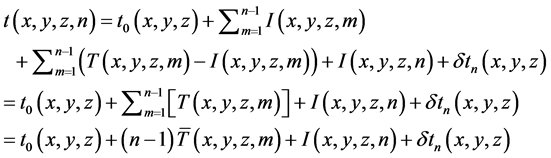
In order to understand why we need to the current theory of time take for example the mechanism of forwarding the time in the analog clock, in which all three hands―second, minute and hour hand―are occupying and leaving their occupies space when the impulse system of the analog clock exerting a single impulse acting on all of them simultaneously, this single impulse is representing superposition of all electromagnetic wave that are reflecting by the surface’s points of underlying elementary constituent matter particle of the clock’s hands and its remainder parts at each exerting epoch of impulse system, however there is existing strong correlation between the number of exerted impulses, the number of occupation epochs of points in the space of motion of the clock’s hands by them and the measurable time by tracking the paths occupied by the analog clock’s hands, we can illustrating this correlation using the fact that the duration of each impulse is one second to write the time t at each point in the space of motion of the specified clock’s hand CH of this analog clock defined with respect to the join points of its hands by during or after the n^th occupation epoch of by CH as the sequence function

seconds, such that is initial leaving epoch of started when the observer starting the tracking of the motion of CH and ending at starting of the first occupation epoch of by CH, for all is representing the number of impulses exerted on CH by the analog clock’s impulse system during the k^th occupation epoch of by CH, for all is representing the summation of the number of impulses exerting after the time on CH during the m^th occupation epoch of by it and the number of impulses exerted on it during the m^th leaving epoch of by it, and is average of

and fulfills

, thus is representing the total lengths of all first occupation epochs of by CH after the time, is representing the total length of all first leaving epochs of by CH occurred between each two occupation epochs of by it after the initial time and is the length of the leaving epoch of by CH elapsed after the end of the n^th occupation epoch of by it, so if the analog clock is ideally perfect then, 3600 or 216,000 in a case of is representing the observable time measurable by tracking the motion second, minute or hour hand respectively, now if we have N identical perfect analog clocks such that for every the point is representing a point in the space of motion of the specified hand of the i^th analog clock defined with respect to the join points of its hands, is representing the number of occupation epochs of by―which is clock hand of the i^th analog clock that we took under consideration, for each

, is representing the number of impulses exerted on it by the impulse system of the i^th analog clock during the k^th occupation epoch of by, for all is representing the summation of the number of impulses exerting on during the m^th occupation epoch of by it and the number of impulses exerting on it during the m^th leaving epoch of by it, and is average of

, and fulfills

then we can define the real time state of this N analog clocks by

, such that seconds where is initial time elapsed during the epoch started when the observer starting the tracking of and ending at starting of the first occupation epoch of by it and is the length of leaving epoch of by elapsed after the end of the occupation epoch of by it, now according to the classical mechanics the time is absolute at all occupation and leaving epochs of epoch of by and then if for all then all second, minute and hour hands of these identical clocks are synchronously occupy their corresponding points in their spaces of motion and synchronously leave them regardless of their spatial distribution or their surfaces orientation in space, and hence the real time state t according to classical mechanics should alwayslied at the equilibrium collinear set, however in general relativity Einstein followed another direction and argued the existence of what is now called the gravitation time dilation [1] which implied that the gravitation field have different value of stress-energy-momentum tensor in different space points occupies by different hands of these analog clocks cause their running at different rates, so according to the general theory of relativity the real time state t may deviating from the equilibrium collinear set as result of difference in gravitation field from one point of space to another point, thus we need mathematical formulation provide a measure to degree to which the real time state of any quantum system consisting of N matter Particles at any points inside their occupies paths from the equilibrium collinear set and all another non-equilibrium collinear set in, the author will approve that each equilibrium or non-equilibrium collinear set is representing vector subspace of, and then if this vector subspaces endowed with usual dot product they will represent vector subspaces of n-dimensional Euclidian space which is representing an inner product Hilbert space.

2.2. The Occupation Epoch Number of the Matter Particle

The occupation epoch number of the matter particle at each space point donated by is representing the number of occupation epochs of by the matter particle with respect to some observer or measurement instrument observing the motion of matter particle during finite observation epoch.

2.3. The Time of the Matter Particle at Each Space Point

If is the occupation epoch number of the matter particle P at the space point then the time of the matter particle P at the space point is defined as the total length of all the occupation and leaving epochs of by the matter particle P and then is defined as following:

(1)

(2)

where: is the length of the initial leaving epoch elapsed before the first occupation of by the matter particle with respect to some observer or measurement instrument observing the motion of matter particle during finite observation epoch.

For each:

is the length of the i^th occupation epoch of by the matter particle.

is the length of the i^th leaving epoch of by the matter particle elapsed aft the i^th occupation epoch.

is the length of the n^th occupation epoch of by the matter particle.

is the length of the epoch elapsed after the end of the n^th occupation epoch of by the matter particle elapsed aft the n^th occupation epoch.

is the average of the time periods:

Important note:

1) The temporal variable is representing a signal indexed by the occupation epoch number.

2) The term is representing a measure of the past temporal epoch before the n^th occupation epoch of by the matter particle, the term is representing the a measure of the present n^th occupation temporal epoch and the term is representing a measure of the future temporal epoch after the n^th occupation epoch of by the matter particle.

2.4. Definition of the Infinitesimal Time as a Function of Infinitesimal Displacement of Space and Occupation Epoch Number

In order to write infinitesimal time as a function of infinitesimal displacement of space and occupation epoch number suppose we have matter particle with rest mass move by speed v with respect to some local observer through some space point at the n^th occupation epoch of by the matter particle, then according to the special relativity theory the momentum of the

particle is given by, where c is the speed of light in vacuum, now

according of the wave-particle duality [6] if is representing the wavelength of this matter particle at the n^th occupation epoch of by it then the momentum of this matter particle is also defined as following:

where h is the Planck’s constant.

→

→

→

→ (3)

where is representing infinitesimal displacement vector of matter

particle at space point, is representing infinitesimal displacement of time and is the component of space metric tensor at the i^th row and the j^th column.

→

→ (4)

Important notes:

From the Equation (3) the speed of matter particle is defined by:

(5)

Thus speed of matter particle should always bounded by the speed of light in vacuum c because:

(6)

For all matter particle possess non-zero mass and occupies non-zero volume of space. Thus we can conclude that the speed of light in vacuum is representing with respect to the current theory is unsurpassable limit for all matter particles possess non-zero mass and occupies non-zero volume of space.

2.5. The Real-Time State of Any Physical System Consisting of N Matter Particles at Specified Space Point

If we have a physical system consisting of N matter particles then the real-time state of this physical system at each space point is defined as following:

(7)

(8)

For all:

where: is the occupation epoch number of the matter particle at

.

is the length of the initial leaving epoch elapsed before the first occupation of by the matter particle with respect to some observer or measurement instrument observing the motion of matter particle during finite observation epoch.

is average time period of the first time periods of at.

is the length of the occupation time of by the matter particle.

is the time elapsed during the matter particle leaving the point after the occupation epoch.

Important notes:

(9)

(10)

(11)

(12)

where:, and

are called hereinafter past, present and future real- time state respectively.

2.6. The Entanglement Translation of Real-Time State of Any Physical System Consisting of N Matter Particles at Specified Space Point

If is representing the real-time state

of some physical system consisting of N matter particles at starting of the occupation of by the matter particle for some then the measurement process of the length of the occupation epoch of by the matter particle that result the

is always transform the real-time state of physical system

according to the following Entangle-

ment Translation:

(13)

For all.

Important note:

1) if the is representing a set of N elementary matter particles then the occupation epoch is infinitesimal thus using the Equation (4) we can write the entanglement translation of as following:

(14)

(15)

2) is representing the normalized reciprocal function of which is normalized by removing the infinity from the range of

reciprocal function.

3) or equi-

valently: which

is always result binary digits indicate wither the matter particle occupied or not and then determine whether the υ^th component of the Real- time state is non-zero covariant under Entanglement Translation or remain zero contravariant, thus the Entanglement Translation is:

I. Pure covariant transformation when for all.

II. Pure contravariant transformation when for all.

III. Mixed covariant and contravariant transformation when and for some.

4) according to this transformation the measurement process of the occupation of by the matter particle that result as observable quantity is the same to the measurement process of the part of leaving of by the rest matter particles of the physical system that are occupied and left, thus the time of each one of these matter particle at of―which is representing the total length of all occupation and leaving epochs of by the matter particle―should increase immediately at the end of measurement epoch, however if some matter particle of the physical system does not occupy from the starting of observation epoch until the starting occupation of by the matter particle then this matter particle will never occupy during the occupation epoch of by the matter particle, and hence the time of this matter particle at―which is representing of total length of all occupation and leaving epochs of by it―will never change from zero during the measurement epoch.

5) For all:

(16)

Which is representing tensor field that take the contravarinat vector and covariant vector

and produce components of the following matrix:

Such that and thus:

(17)

Such that: is equivalent to the number of non-zero components of and the Real-time state

.

Now:

→

such that

→

such that is N × N identity matrix

→ (18)

Thus the Entanglement Translation:

is translational invariant with respect to the operator.

2.7. The Real-Time Digital State of the N Matter Particles Physical System at Specified Space Point

If is representing the real-time state

of some physical system consisting of N matter particles at

then the Real-time digital state at that is corresponding to is defined as following:

(19)

Important note:

1) The value of indicate wither the matter particle occupied the point or not with respect to observer or measurement instrument tracking its motion of through.

2) If is representing the real-time

state of the physical system at starting of the occupation of by the matter particle for some and is the result of the measurement process of the length of the occupation epoch of

by the matter particle then the Entanglement Translation of

is given as following:

Such that

(20)

Thus the Real-time digital state is representing the base state of Entanglement Translation of the real-time state

.

However

which is

consisting of N-tuples of binary digits thus the Real-time digital state

as well as Entanglement Translation

are quantifying the motion of the constituent matter particles of the physical system through, this quantification allow these matter particles move exclusively at a finite sequential set of digital levels defined in the following section.

3)

where:

and:

Thus we can write the Entanglement Translation of:

Such that

As following:

(21)

(22)

(23)

(24)

2.8. The Digital Levels of Real-Time Digital States of the Physical System Consisting of N Matter Particles

For any physical system S consisting of N matter particles and for all the digital level n of S is defined as the set of all possible real-time digital states of S at any space point consisting of n components equivalent to one and rest components equivalent to zero, thus if is representing the set of all subsets of that are consisting of n ele-

ments, and for any set A and B then the n^th digital level of S

is defined as following:

(25)

which their element are defined as surjective function such that for each:

(26)

Important note:

1) If is repre-

senting the real-time digital state of some physical system consisting of N matter particles at, then there exists:

and fulfills:

2) If is real-time digital state of some physical system consisting of the matter particles at then before the first occupation epochs of by any matter particle belong to

―with respect to some observer or measurement instrument tracing the motion of the matter particles through― the real-time digital state of the of the physical system at is equivalent to the equilibrium state

called herei-

nafter the falsehood digital state at which is representing the unique element of the digital level 0 of the system, then this state either stay in the digital level 0 along the observation epoch of the physical system or change due the occupation of by one matter particle belong to

to one state in the digital level 1 which is level consisting of all real-time digital states with one components equal one and rest components equal zero, then this state either stay in the digital level 1 or change due the occupation of by new one matter particle belong to to one state in digital level 2 which is level consisting of all digital states with two components equal one and rest components equal zero, and so on until the digital state of the physical system reach the stationary equilibrium digital

state at the digital level N and then resisting at

this digital state for rest of observation epoch of the physical system. However we must keep in mind the impossibility of transition the Real-time digital state to another Real-time digital state belong to the same or lower digital level or to another Real-time digital state belong to higher digital level with i^th component equivalent to zero for all fulfill because each components of the digital state can only change from zero to one when some matter particle of the physical system start its first occupation epoch, Figure 1 representing an explanation of distribution of real-time digital states of any physical system consisting of 4 matter particles over their corresponding digital levels in addition to the possible transition of the Real-time digital states from different digital states to the Real-time digital states distributed in their near higher digital level.

3) If the constituent matter particles of the physical system are distributed into set of finite orbits such as the distribution of electrons in atoms then for each one of these orbits the real-time digital state of the physical system at each space point belong to it will be the same when all matter particles at that orbit occupy all space points belong to it, however this symmetry of digital states at that orbit can break by the jumping of one matter particles to that orbit which can transit all points occupied by it at that orbit to the same digital state belong to next higher digital level, thus the distribution of the constituent

Figure 1. Illustration of digital levels and all possible transition between the real-time digital states belong to them for any physical system consisting of 4 matter particles.

matter particles into set of finite orbits is equivalent to the distribution of it into set of finite digital levels such that jumping of matter particle from initial orbit to the final orbit is equivalent to the transition of digital states at all points occupied by it at the final orbit to the same real-time digital state belong to next higher digital level.

2.9. The Real-Time Transition State

For any physical system S consisting of N matter particles the real-time transition state of the physical system at that is corresponding to its real-time digital state at:

is defined as the superposition of all

real-time digital states at that the physical system can transit to it at the of the next occupation epochs of by one of its constituent matter particles which is defined as following:

(27)

Fulfills:

(28)

(29)

For all fulfills.

Such that:

(30)

(31)

fulfills and for all fulfills.

where: is the tensor product (outer product) operation.

and are normalized reciprocal

transpose of and respectively which are defined by taking the normalized reciprocal of the components of transpose of and respectively.

Important note:

1) When the physical system at the real-time digital state:

the next occupation epochs of

by one of its constituent matter particles P is either leaves the physical system at the real-time digital state in a case that P occupied at the previous occupation epoch or transit the real-time digital state to some state at the next higher digital level such that fulfills

, thus the real-time transition state is defined as superposition of its current real-time digital state and all real-time digital states at the next higher digital level that the physical system that can transit to them.

2) For all the components of and at the i^th row

and the j^th column which are and

respectively indicate wither both the matter particles and occupied or not, thus and can play the role of observables operators that the Hermition matrices played in quantum mechanics because they are either leave the physical system at its current real-time digital state or transit it to one real-time digital state in next higher digital level when they act on the real-time transition state, however we use the normalized reciprocal as involution function instead of complex conjugate that used in quantum mechanics, so and are equal to their normalized reciprocal transposes in same way that the Hermition matrices equal to their complex conjugate transposes. In computation term and are representing irreversible gates that forward the time of each constituent particles of the physical system only at the direction of increasing the number of occupation and leaving epochs of space points by it.

3) we can calculate the coefficients and as following:

Since for all and:

the conditions:

Implied that:

And then:

So if are representing the elements of

for some integer then:

And:

→

Now there is two possible cases of above linear system depend on the value of n defined as following:

A. if n = 0 then the linear system is reduced to:

And then:

B. If n > 0 then above linear system is defined in matrix form as following:

Thus using the Cramer’s rule [3] for solving the linear system we find:

And hence the real-time transition state is defined as following:

(32)

2.10. The Analog Occupies Path of the Physical System Consisting of N Matter Particles

The analog occupies path of N matter particles physical system is the path that consisting of all real-time states at all space point occupied or occupies at least by one of its constituent matter particles.

2.11. The Digital Occupies Path of the Physical System Consisting of N Matter Particles

The digital occupies path of N matter particles physical system is the path that consisting of all real-time digital states at all space point occupied or occupies at least by one of its constituent matter particles.

3. Mathematical Formulation: An Introduction to the Calculus of Fluctuation

3.1. The n-Dimensional Real Collinear Set

For each the n-dimensional real collinear set of any two point donated by is defined as a set of all point in lied at the line that contains p and q.

Example of real collinear set

The set of real numbers is a 1-dimesional collinear set of any two real number x, y. i.e.,.

3.2. The n-Dimensional Displacement Vector

For all and the n-dimensional displacement vector from p to q is defined as following:

(33)

Important note:

For all the author will donate to the vector

by such that.

3.3. The Equilibrium Null Point and Vector

The equilibrium null point is the point is the point and the

equilibrium null vector is vector.

3.4. The Equilibrium Unity Point and Vector

The equilibrium unity point is the point and the equili-

brium unity vector is the vector.

3.5. Conditions of Positioning in n-Dimensional Collinear Set

For each the n-dimensional real collinear set of any two point such that and the conditions of positioning in are defined as following:

1) The tangent and cotangent of the angle between the line that connect x and q should be equal to the tangent and cotangent of the angle between the line that connect x and y, mathematically this condition is defined as following:

satisfy and.

2) The equivalent components of x and y should be equivalent to their corresponding components of q, mathematically this condition is defined as following: fulfills.

Important note:

From the first condition satisfy and

Also

From the second condition satisfy we find that

Also

→

→ (34)

3.6. The n-Dimensional Collinear Vectors Set

If is n-dimensional real collinear such that then the collinear vectors set of donated by is the set of all displacement vectors in that their heads are belonging to and tails are equivalent to the equilibrium null point, which is defined as following:

(35)

Important note:

For any the exists displacement vector

with components equivalent to thus for all

fulfill: such that and because: and the components of

and are equivalent to the components of and respectively.

3.7. Theorem (3.2)

For all the n-dimensional displacement vector set

is representing vector subspace of and is repre-

senting subgroup of.

Prove:

For all, all fulfills, all

and all such that:

and

:

1).

2) (Closure under ad-

dition and scalar multiplication).

3) (Associativity of addition).

4) (Commutatively of

addition).

5) (Identity element of addition).

6) fulfills

(Inverse element of addition).

7) (Compatibility of scalar multiplication with field

multiplication).

8) (Distributivity of scalar multiplication with respect to vector addition).

9) (Distributivity of scalar multiplication with respect to field addition).

10) (Identity element of scalar multiplication).

3.8. The n-Dimensional Real State Space

For all such that the n-di- mensional real state space at x is the vector subspace of defined by

and endowed with inner product

such that for all and

:

Important note:

is representing vector subspace of n-dimensional Euclidean

space thus is representing inner product Hilbert space.

3.9. Equilibrium and Non-Equilibrium Classification of n-Dimensional Real State Space

For all we can classify the n-dimensional real state

space as:

1) Equilibrium n-dimensional real state space in a case of for all.

2) Non-Equilibrium n-dimensional real state space in a case of for some.

Important notes:

If is equilibrium n-dimensional real state space then:

3.10. The Normalized Reciprocal of Real Scalar

For any the normalized reciprocal of x is defined as following:

Important note:

1) is called normalized reciprocal because the usual reciprocal of x which is

equal is contain infinity in his range when, so it is normalized by

removing this infinity from its range:

2) is representing binary digit.

3) The Dirac’s delta function is related to normalized reciprocal as following:

(36)

Which is equal zero at all and one at.

3.11. The Normalized Reciprocal Transpose of the Matrix

For any matrix the normalized reciprocal of

is defined as following:

(37)

3.12. Signal Tensor Field

At any point the signal tensor field is second order ten-

sor that take from and its corresponding dual vector from such that and produce components

defined as following:

(38)

Or in tensor notation:

(39)

For all.

Important notes:

1) For all the μ^th diagonal component of which is equal is corresponding to the μ^th components of the binary digital state binary state so the diagonal components of are representing the digital components of it, and all the rest components of for all are representing the analog normalized ratio between the components of at different indices.

2) For all if then for all

so in the signal tensor field the present and absent of the digital signal is restricted by the present and absent of its corresponding analog signals and vice versa.

3) at all point because for all fulfill and

thus:

(40)

4)

→ ( 41)

or in tensor notation:

(42)

For this reason will play in the digital matter particle Physics the similar role that Herniation matrix or in general adjoin operator plays in quantum physics.

5) For all the vector:

→ (43)

Such that is equivalent to the digital level of the digital state

.

In tensor notation this equation is given as following:

(44)

3.13. The Fluctuation Tensor Field

The fluctuation tensor field is representing bilinear map ―such that is the space of all square matrix―defined for all

and as following:

(45)

Such that is the outer product (tensor product) operation [2] defined as following:

(46)

and

(47)

Thus If and then the fluctuation tensor field of x and y donated by is the set of ordered real numbers called its components indexed by such that

and defined as following:

(48)

The Properties of commutator tensor field:

a Anti-symmetric because:

b Alternating because:

c Non-degenerate because:

For every there exists and fulfills, and implied:

Because

d Bilinear because for all, , , and all:

.

Thus.

Also.

Thus.

3.14. Theorem 3.3

If, then the fluctuation tensor is representing a measure of degree to which the point x and y deviate from belonging to the collinear set and respectively because:

1) for all vanished when there is no deviation.

2) for all and

i.e. the fluctuation tensor field is a invariant under parallel translation of with respect to the line that all elements of lie or parallel translation of with respect to the line that all elements of

lie. Thus all element lie at single line parallel to the line that all elements of some collinear set S lie have a same measure of deviation from belonging to S defined as fluctuation tensor field.

Prove:

1) for all and all fulfill:

and hence:

→

2) For all, and all:

Thus if and then there exist four points

, ,

, fulfill

, and for all fulfill

and and all fulfill and:

→

→

For all:

→

3.15. The Spin’s Fluctuation Tensor Field at Each Matter Particle’s Surface Point

The spin fluctuation tensor field is defined at each surface point of any matter

particle resisting with respect to an arbitrary observer at the position

as following:

(49)

where: is linear and momentum vector of the matter particle.

Important note:

Each components of the spin’s fluctuation tensor field is corresponding to either positive or negative components of angular momentum vector:

and vice versa, so the

components of the spin’s fluctuation tensor field are vanishes― becomes zero―when all component of are vanishes and vice versa, also the components of the spin’s fluctuation tensor field are conserved when the components of are conserved and vice versa, those two strong correlated feature between the components of the spin’s fluctuation tensor field and the components of allow the author to introduce the following theorem.

3.16. Theorem 3.5: Spin’s Fluctuation Theorem

Any matter particle P possesses a non-zero mass m can possess:

1) A non-zero spin angular momentum at arbitrary time interval if and only if all surface points of P are not moving in the same direction of its position vector during this time interval.

2) A conserved spin angular momentum at any two arbitrary time intervals and if and only if any surface points of P donated by s located with respect to an arbitrary observer or measurement instruement at

the position at the time t fulfills:

(50)

where:

i) is infinitesimal displacement of s at the time interval.

ii) is infinitesimal displacement of s at the time interval .

Prove:

1) Suppose we have some arbitrary surface point of P resisting with respect to

an arbitrary observer at the position at the time t.

Now the spin angular momentum of P at is defined as a cross product of

and the linear momentum vector as following:

In other hand the spin’s fluctuation tensor field is defined as following:

Thus every component of is equivalent to either positive or negative value of one component of, so all components of vanishes―becomes zero―when all components of vanishes.

Now the infinitesimal displacement vector, thus the fluctuation

tensor field of and is defined using bilinearity property of fluctuation tensor field as following:

→

Because is representing infinitesimal non-zero change of time, the spin’s fluctuation tensor field vanishes―and then the spin angular momentum vector―when all components of the fluctuation tensor field

vanishes so according to the theorem 3.2 vanishes when or equivalently when. Thus the matter

particle P possesses a non-zero spin angular momentum if and only if all surface points of P are not moving in the same direction of their position vectors.

2) Lets represents a surface point of P resisting with respect to an arbitrary ob-

server at the position at the time t, let is

representing the infinitesimal displacement of the matter particle’s surface

points during the time interval, is the position

of the matter particle’s surface point s at the time, and let

is representing the infinitesimal displacement of

the matter particle’s surface points during the time interval, now the spin angular momentum vectors of the matter particle at s during the time interval and and donated by and respectively are given as following:

Also the spin’s fluctuations tensor fields of the matter particle at s during the time interval and and donated by and respectively are given as following:

Thus every component of is equivalent to either positive or negative value of one component of and every component of is equivalent to either positive or negative value of one component of, so if and only if and then if and only if:

or equavently if and only if:

or equivently if and only if:

Because

and

,

if and only if:

Important Notes:

1) The first part of the above theorem implied that if the matter particle possesses non-zero mass and non-zero spin angular momentum then it’s all surface points should move in different direction of all position vectors defined with respect to all observers observing them, thus the first part of the above theorem approve that the non-zero spin angular momentum of any matter particle possesses non-zero mass is intrinsic property independent from the observer’s localization with respect to its surface point.

2) The second part of the above theorem illustrate the relation between spatial and temporal coordinates of the surface points of any matter particle possesses non-zero mass and conserved spin angular momentum.

3.17. Theorem 3.6

If, ,

and such that, , is not parallel to and then and are intersected at the point fulfills:

1)

(51)

For all and all fulfill

.

2) if and for some

fulfill and, and some and

fulfill, , for all―i.e. is not parallel to―and either or, then:

(52)

For all and all fulfill.

Prove:

Suppose we have, ,

and such that, , and is not parallel to, suppose that is intersection point of and

: Now for all fulfills, and either

or―i.e.:

(a)

and

(b)

→

→

→

→ (c)

(d)

Now by substituting from Equation (c) into Equation (d) we find:

→

→

→

(e)

Now from Equation (a):

For all.

→

→ (f)

Now by substituting from Equation (e) into Equation (f) we find:

→

→

→

For all and all fulfill, and either or.

This proves the first part of the theorem, now to prove the second part we can use the first proved part as following:

→

→

→

Thus if and for some

fulfill and, and some and

fulfill, , for all―i.e. is not parallel to―and either or, then:

→

→

For all and all fulfill, and either or.

This equation is representing the fundamental fluctuation tensor field equations which are invariant under any arbitrary change of, and by any

, and respectively

such that for all, thus:

For all and all fulfill, and either or.

3.18. Orthogonal n-Dimensional Real Collinear Sets

For each the two collinear sets and are called orthogonal if and only if:

1).

2), for all and.

Such that donate to the dot product of and.

3.19. N-Dimensional Real Collinear Sets Space

The n-dimensional real collinear sets local space at donated by is the space of all n-dimensional real collinear sets intersected at the point t, which is given as following:

Important note

Any is representing the origin of fulfills for any

two collinear sets and belong to

, such that, , fulfill for all

―i.e. is not parallel to―and fulfill and the equations:

For all and all fulfills, and either or, these equations are invariant under any arbitrary change of and.

3.20. The n-Dimensional Real Collinear Sets Bundle

The n-dimensional real collinear sets bundle is the union of all n-dimensional real collinear sets spaces at all points in which is given as:

(53)

3.21. The n-Dimensional Real Coplanar Set

For all the n-dimensional coplanar set of p, q and r donated by is a set of all point in lied at the n-dimensional plane contains p, q and r, which is defined as following:

(54)

3.22. The n-Dimensional Real Coplanar Space

The n-dimensional real coplanar space at each point donated by is defined as following:

(55)

Important notes:

is defined as the space of all coplanars that are containing some point represents intersection point of collinear sets then using the theorem (3.6) we find:

(56)

For all and all fulfills

, and

.

3.23. The n-Dimensional Real Coplanar Bundle

The n-dimensional real coplanar bundle is union of all n-dimensional real coplanar spaces at all space point in which is defined as following:

(57)

3.24. The N-Dimensional Real Space-Time

For any physical system consisting of N matter particles, the N-dimensional real space-time is the section of N-dimensional real coplanar bundle that consisting of all real-time states of the physical systems at each all space point occupied by one or more constituent matter particles of the physical system during finite epoch with respect to an arbitrary observer. Thus if then at each space point occupied by one or more constituent matter particles of the physical system the real-time state of the physical system is representing an element of the section of that defined as following:

(58)

Important notes:

If the real-time state of the physical system at the space point occupied by one or more constituent matter particles of it is defined according to the equation 9 as following:

,

then there exist at least in principle fulfill

, ,

and

(59)

4. Conclusion

As the spatial coordinates x, y and z which are representing the lengths between origin () and (), () and () respectively, the time coordinate is representing the total length of all occupation and leaving epochs of space point including the length of the initial leaving epoch elapsed before the first occupation of space point by the matter particle during finite observation epoch, this implied that the direction of time of any matter particle at each space point P occupied by it is the direction of increasing the number of occupation and leaving epochs of P by it, and the measurement of occupation of space point by one constituent matter particles of the physical system produce the same measurement of the time of the rest matter particles of the physical system that occupied and left the space point during finite observation epoch regardless of their distribution in space, this give simple reinterpretation of quantum entanglement. The motion of the constituent matter particles on separated orbits is equivalent to their motion in separated digital levels, and their transitions from one orbit to another one is equivalent to their transition from one digital level to another.

Acknowledgements

Thanks for my father who supported all my education levels and for my wife Ayaat Ahmed Osman for here incorporeal support for me in scientific papers publications.

Conflicts of Interest

The authors declare no conflicts of interest.

References

[1]	Einstein (1916) The Foundation of the Generalized Theory of Relativity. https://en.wikisource.org/wiki/The_Foundation_of_the_Generalised_Theory_of_Relativity
[2]	Einstein, Podolsky and Rosen (1935) Can Quantum-Mechanical Description of Physical Reality Be Considered Complete?
[3]	Bell, J. (1964) Physics, 1, 195-200.
[4]	McTaggard, J.E. (1908) The Unreality of Time. https://docs.google.com/viewer?a=v&pid=sites&srcid=ZGVmYXVsdGRvbWFpbn x0eXNnc2l0ZXxneDozYmE1OWUyMGU0NjU1YzE4
[5]	Quantum Experiment Shows How Time “Emerges” from Entanglement. https://medium.com/the-physics-arxiv-blog/quantum-experiment-shows-how-time- emerges-from-entanglement-d5d3dc850933#.733j5z1ez
[6]	New Quantum Theory Could Explain the Flow of Time. WIRED. Retrieved 13 October 2014.