Study of Even ^230-238U Isotopes by Using Cranked Nilsson Model, Single Particle Schrodinger Fluid and Collective Model

K. A. Kharroube

Mathematics Department, Faculty of Science, Lebanese University, Beirut, Lebanon.

DOI: 10.4236/ojm.2017.72003                

Abstract

The Cranking Nilsson model is applied to calculate the single-particle energy eigenvalues and eigenfunctions of nuclei in a strongly deformed potential. Accordingly, The L. D. Energy, the Strutinsky inertia, the L. D. inertia, the volume conservation factor , the smoothed energy, the BCS energy, the G-value and the electric quadrupole moment of the five uranium isotopes: ²³⁰U, ²³²U, ²³⁴U, ²³⁶U and ²³⁸U are calculated as functions of the deformation parameter. Furthermore, the single-particle Schrodinger fluid is applied to calculate the rigid-body model, the cranking-model and the equilibrium-model moments of inertia of the five uranium isotopes. Moreover, the collective model is applied to calculate the rotational energies of these isotopes. The best potential and deformation parameters are also given.

Keywords

Deformed Nuclei, Cranked Nilsson Model, Single-Particle Schrödinger Fluid, Collective Model, Quadrupole Moment, Moment of Inertia, Rotational Energy Levels, Uranium Isotopes

1. Introduction

As we go far from closed shells, some new very simple and systematic features start to show up for some nuclei. This is true for nuclei with mass number A in the range, for, for nuclei in the s − d shell and for p shell nuclei in. Even-even nuclei in the same region all have a low-lying first excited state with and electric quadrupole radiation is strongly enhanced. A description of these nuclei and many other deformed nuclei has been given by a model proposed and developed by A. Bohr and B. Mottelson [1] . The success of the independent-particle approximation for spherical nuclei near closed shells naturally suggests adopting a similar procedure for deformed nuclei. Thus, as a first guess for the deformed nucleus internal wave function we want to take an independent-particle wave function, generated from a deformed potential. One of the most successful models for generating realistic intrinsic single particle states of deformed potentials is that first proposed by Nilsson [2] . This model was limited to nuclei with axially symmetric quadrupole deformations. Positive values of the deformation parameter correspond to prolate deformation and negative values to oblate deformation.

The success of the description of many nuclei by means of deformed potential can be taken as an indication that by distorting a spherical potential in this manner we automatically obtain the right combination of spherical eigenfunctions that makes the corresponding Slater determinant a better approximation to the real nuclear wave function. From this point of view, the deformed potential is a definite prescription for a convenient mixing of various configurations of the spherical potential. The absolute values of the rotational energies or equivalently the moments of inertia require the knowledge of the fine details of the intrinsic nuclear structure. Consequently, the investigation of the nuclear moments of inertia is a sensitive check for the validity of the nuclear structure theories [3] .

Theoretical investigations of Ref. [4] on rare earths and actinides showed that, having reproduced the experimental equilibrium deformations of nuclei, one was able to reproduce their experimental moments of inertia. More specifically, using the cranking formula and a realistic model of intrinsic structure of a nucleus (realistic single-particle potentials plus pairing interaction), one was also able to reproduce the experimental ground state moments of inertia within the limits of 10% - 25%.

It is well known that nearly all fully microscopic theories of nuclear rotation are based on or related in some way to the cranking model, which was introduced by Inglis [3] in a semi-classical way, but it can be derived fully quantum mechanically, at least in the limit of large deformations, and not too strong K-admixtures. The cranking model has the following advantages [3] [5] .

1) In principle, it provides a fully microscopic description of the rotating nucleus. There is no introduction of redundant variables, therefore, we are able to calculate the rotational inertia parameters microscopically within this model and get a deeper insight into the dynamics of rotational motion.

2) It describes the collective angular momentum as a sum of single-particle angular momenta. Therefore, collective rotation as well as single-particle rotation, and all transitions in between such as decoupling processes, are handled on the same footing.

3) It is correct for very large angular momenta, where classical arguments apply.

A simple and widely used way to describe the change of the single-particle structure with rotation is given by the Cranked Nilsson model (CNM) [5] - [10] . It is the method of calculating the shell correction energy that made it possible to do large-scale calculations where the nuclear potential-energy surface was explored in great details as a function of different deformation degrees of freedom. Important achievements in this field include the prediction of Super deformed high-spin states and terminating bands. The CNM model is a theoretical approach that provides us with good physics interpretation of the different properties of deformed nuclei and at the same time allows us to carry out systematic and accurate calculations of the different properties of the deformed even-even nuclei.

In addition to individual nucleons changing orbits to create excited states of the nucleus as described by the shell model, there are nuclear transitions that involve many (if not all) of the nucleons. Since these nucleons are acting together, their properties are called collective, and their transitions are described by a collective model [1] [3] of nuclear structure. Nuclei with high mass number have low-lying excited states which are described as vibrations or rotations of non- spherical nuclei. Many of these collective properties are similar to those of a rotating or vibrating drop of liquid, and in its early development the collective model was called the liquid-drop model. The collective model, also called unified model, describes the nuclei in such a way that they incorporate aspects of both the nuclear shell model and the liquid-drop model in order to explain certain magnetic and electric properties that neither of the two separately can explain. In the collective model, high-energy states of the nucleus and certain magnetic and electric properties are explained by the motion of the nucleons outside the closed shells (full energy levels) combined with the motion of the paired nucleons in the core. The increase in nuclear deformation that occurs with the increase in the number of unpaired nucleons accounts for the measured electric quadrupole moment, which may be considered as a measure of how much the distribution of electric charge in the nucleus departs from spherical symmetry.

The study of the velocity fields for the rotational motion led to the formulation of the concept of the Schrödinger fluid [11] [12] [13] [14] . The problem of a single quantum particle moving in a time-dependent external potential well is formulated specifically to emphasize and develop the fluid dynamical aspects of the matter flow in this concept. This idealized problem, the single-particle Schrödinger fluid, is shown to exhibit already a remarkably rich variety of fluid dynamical features, including compressible flow and line vortices. It provides also a sufficient framework to encompass simultaneously various simplified fluidic models for nuclei which have earlier been postulated on an ad hoc basis, and to illuminate their underlying restrictions. Explicit solutions of the single-par- ticle Schrödinger fluid problem are studied in the adiabatic limit for their mathematical and physical implications (especially regarding the collective kinetic energy).

Sadiq et al. [15] used the projected shell model to study the yrast positive parity bands in ^230?240Unuclei. The energy levels, deformation systematics, E2 transition probabilities and g-factors are calculated. The calculation reproduces the observed positive parity yrast bands and B(E2) transition probabilities. The observed deformation trend of low-lying states in Uranium nuclei depends on the occupation of down-sloping components of high j orbits in the valence space. The low-lying states of yrast spectra are found to arise from 0-quasiparticle (qp) intrinsic states, whereas the high spin states possess multi-qp structure.

Doma, Kharroube, Tefiha and El-Gendy [16] have recently applied the CNM, the concept of the single-particle Schrödinger fluid and the nuclear superfluidity model to calculate the electric quadrupole moments and the moments of inertia of the even-even p-and sd-shell nuclei and the obtained results are in good agreement with the available experimental data. Furthermore, Doma and El- Gendy [17] applied the collective model to calculate the rotational and vibrational energies of the even-even ytterbium: ¹⁷⁰Yb, ¹⁷²Yb and ¹⁷⁴Yb, hafnium: ¹⁷⁶Hf, ¹⁷⁸Hf and ¹⁸⁰Hf and tungsten: ¹⁸²W, ¹⁸⁴W and ¹⁸⁶W nuclei. Moreover, they have applied the single-particle Schrödinger fluid to calculate the nuclear moment of inertia of the nine mentioned nuclei by using the rigid-body model and the cranking model. Furthermore, they applied the CNM to calculate the L. D. energy, the Strutinsky inertia, the L. D. inertia, the volume conservation factor, the smoothed energy, the BCS energy, the G-value, the total ground- state energy and the quadrupole moment of the nine mentioned nuclei as functions of the deformation parameters and.

In the present paper, we applied the concept of the single-particle Schrödinger fluid to calculate the cranking-, the rigid body- and the equilibrium-models moments of inertia for the five uranium isotopes: ²³⁰U, ²³²U, ²³⁴U, ²³⁶U and ²³⁸U. Furthermore, we applied the CNM to calculate the L. D. energy, the Strutinsky inertia, the L. D. inertia, the volume conservation factor, the smoothed energy, the BCS energy, the G-value and the electric quadrupole moment of the mentioned five isotopes. Moreover, we applied the collective model to calculate the rotational energies of the five uranium isotopes. Variations of the calculated characteristics with respect to the deformation parameter β and the nonaxiality

parameter γ, which are assumed to vary in the ranges and are carried out.

2. The Cranked Nilsson Model

2.1. The CNM Hamiltonian

The single particle Hamiltonian in the CNM assumes the form [4] [5] [17]

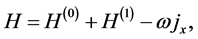(2.1)

where

(2.2)

Here, the oscillator parameters and assume the form [18]

(2.3)

The second term in the right-hand side of Equation (2.1) is given by

(2.4)

In the above equations is the deformation parameter which is related to Nilsson’s deformation parameter [2] by, γ is the nonaxiality

parameter and refers to the hexadecapole deformations degree of freedom. The angular frequency is given in terms of the non- deformed frequency by [4]

(2.5)

The non-deformed oscillator parameter is given in terms of the mass number A and the number of protons Z by [19]

(2.6)

The stretched square radius is written in the form

(2.7)

The hexadecapole potential is defined to obtain a smooth variation [4] [5] [6] in the γ-plane so that the axial symmetry is not broken for and. It is of the form

(2.8)

where the parameters are chosen as

and

(2.9)

In Equation (2.9) t refers to the stretched coordinates, etc.

The Hamiltonian can be simplified to

(2.10)

Hence, to the first order in, the Hamiltonian takes the form

(2.11)

where

(2.12)

Also, direct substitution for the different quantities in the operator gives

(2.13)

2.2. The Single Particle Energy Eigenvalues and Eigenfunctions of the CNM

The method of finding the energy eigenvalues and eigenfunctions of the Hamiltonian H, Equation (2.1), can be summarized as follows:

1) Solving the Schrödinger’s equation of the Hamiltonian (2.10)

(2.14)

exactly.

2) Modifying the functions to become eigenfunctions for the solutions of the corresponding equation for

3) Using the functions obtained in step 2) to construct the complete function, the eigenfunction of the Hamiltonian H, in the form of linear combinations of the above functions, as basis functions, with given total angular momentum j and parity π.

4) Constructing the Hamiltonian matrix H by calculating its matrix elements with respect to the basis functions defined in step 3).

5) Diagonalizing the Hamiltonian matrix H to find the energy eigenvalues and eigenfunctions as functions of the non-deformed oscillator parameter and the parameters of the potentials.

2.3. The solutions of Equation (2.14)

The solutions of the equation are given, with the usual notations, by [16] [17]

(2.15)

(2.16)

where are the normalized spherical harmonics with and is the nucleon orbital angular momentum quantum number.

The radial wave functions are given by

(2.17)

where, and the number of quanta of excitation N is related to the orbital angular momentum quantum number by or 1.

The last function in the right-hand side of Equation (2.17) is the associated Laguerre polynomial. Since the nucleon has spin and intrinsic spin wave functions, where, the single particle wave functions of the Hamiltonian are, then, given by

(2.18)

The classifications of the functions are straightforward.

2.4. The Eigenfunctions of the Hamiltonian

Wave functions with given values of the number of quanta of excitations N, the orbital angular momentum quantum number, the total angular momentum J and the parity π can be constructed from the functions (2.18), in the usual manner, as follows

(2.19)

The functions are used as basis functions for the construction of the single particle nuclear wave functions with given total angular momentum J and parity π, in the usual manner, as follows

(2.20)

Accordingly, we obtain 15 wave functions, states, namely

The classifications of these states in terms of the functions are straight- forward.

The matrix elements of the Hamiltonian with respect to the functions (2.20) are given by

(2.21)

It is easy to show that the matrix elements of the operator with respect to the basis functions are given, with the usual notations by

(2.22)

where and.

Also, the matrix elements of the spherical-harmonic operators and with respect to the functions (2.15) are straightforward.

2.5. Total Nuclear Quantities

We define the total energy by [4] [5] [6]

(2.23)

where the single-particle spin contribution is obtained as

(2.24)

The summations in (2.23) run over the occupied orbitals in a specific configuration of the nucleus. The shell energy is now calculated from

(2.25)

where

(2.26)

and is the smoothed single-particle sum which can be evaluated according to the Strutinsky prescription [6] [20] . The detailed formulas for are discussed in [21] for and in [22] for.

The pairing energy is an important correction that should decrease with increasing spin and becomes essentially unimportant at very high spins. To obtain an () average pairing gap ∆, which varies as, the pairing strength G is chosen as [8] [9] [10] .

(2.27)

with g₁/g₀ ≈ 1/3. Furthermore, the number of orbitals included in the pairing calculation should vary as and for protons (p) and neutrons (n), respectively. If pairing is calculated, the pairing strength G is an important parameter. Its value is given according to (2.27). As a default, we use [5] .

The total nuclear energy is now calculated by replacing the smoothed single- particle sum by the rotating-liquid-drop energy and adding the pairing correction

(2.28)

or

where, is liquid drop energy, is the smooth moment of inertia factor,. The shell and pairing energies are evaluated separately for protons and neutrons at, while the renormalization of the moment of inertia introduces a coupling when evaluating for.

From the single-particle wave functions, the electric (or mass) quadrupole moment may be calculated as

(2.29)

where for protons and 0 for neutrons. For more details concerning the Cranked Nilsson model, see [6] .

3. The Single Particle Schrödinger Fluid

The problem of a single quantal particle moving in a time-dependent external potential well was formulated specifically to emphasize and develop the fluid dynamical aspects of the matter flow [11] [12] . This idealized problem, the single-particle Schrödinger fluid, is shown to exhibit already a remarkably rich variety of fluid dynamical features, including compressible flow and line vortices. It provides also a sufficient framework to encompass simultaneously various simplified fluidic models for nuclei and to illuminate their underlying restrictions. Accordingly, each nucleon in the nucleus is assumed to move in a single- particle potential, which is deformed with time t, through its parametric dependence on a classical shape variable. Thus, the Hamiltonian for the present problem is given by [11] [12]

(3.1)

The single-particle wave function, which describes the motion of a nucleon, satisfies the time-dependent Schrödinger equation

(3.2)

We use polar form of the wave function and isolate the explicit time dependence in by an energy phase factor, i.e. we write [11] [12]

(3.3)

where is the intrinsic energy of the nucleon that depends on time through α. Then, we write the complex wave function in polar form

(3.4)

where and are assumed to be real functions of and.

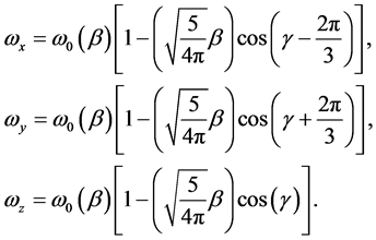
The average potential field is assumed to be in the form of anisotropic harmonic oscillator potential. The intrinsic energy of the single particle state is, then

(3.5)

In terms of the frequencies and we introduce one single parameter of deformation given by [2]

(3.6)

(3.7)

Applying the time-dependent perturbation method and using the equation arising from the first-order perturbation of the wave function we can calculate the first-order time-dependent perturbation correction to the wave function explicitly as function of the number of quanta of excitations corresponding to the Cartesian coordinates and the quantity, defined by [11] [12]

(3.8)

which is a measure of the deformation of the potential.

We use the cranking-model formula for the calculation of the moment of inertia. After the inclusion of the residual pairing interactions by the quasiparticle formalism, the formula for the x-component of the moment of inertia is given in terms of the matrix elements of the single-particle angular-momentum operator corresponding to the rotation around the intrinsic x-axis, the variational parameters of the Bardeen-Cooper-Sehrieffer wave function corresponding to the single particle states and the quasiparticle energy of this state [23] .

We now examine the cranking moment of inertia in terms of the velocity fields. Bohr and Mottelson [1] showed that for harmonic oscillator case at the equilibrium deformation, where

(3.9)

the cranking moment of inertia is identically equal to the rigid moment of inertia:

(3.10)

We note that the cranking moment of inertia and the rigid moment of inertia are equal only when the harmonic oscillator is at the equilibrium deformation. At other deformations, they can, and do, deviate substantially from one another [12] .

The following expressions for the cranking-model and the rigid-body model moments of inertia, and, are obtained [12] :

(3.11)

(3.12)

where E is the total single particle energy, given by (3.5) and q is the ratio of the summed single particle quanta in the y-and z-directions

(3.13)

q is known as the anisotropy of the configuration. The total energy E and the anisotropy of the configuration q are easily calculated for a given nucleus with mass number A, number of neutrons N and number of protons Z. Accordingly, the cranking-model and the rigid-body model moments of inertia are obtained as functions of the deformation parameter β and the non-deformed oscillator parameter by suitable filling of the single-particle states corresponding to the ground-state of the given nucleus [13] [14] .

4. The Collective Model

The two most important developments in nuclear physics were the shell model and the collective model. The former gives the formal framework for a description of nuclei in terms of interacting neutrons and protons. The latter provides a very physical but phenomenological framework for interpreting the observed properties of nuclei. A third approach, based on variational and mean-field methods, brings these two perspectives together in terms of the so-called unified models. Together, these three approaches provide the foundations on which nuclear physics is based. They need to be understood carefully, in order to gain an understanding of the foundations of the models and their relationships to microscopic theory as given by recent developments in terms of dynamical symmetries.

On the basis of the collective model, we calculated the rotational energies by using the following formula [17]

(4.1)

where A is the reciprocal-moment of inertia of the nucleus,. The value of A has been determined for all the considered uranium isotopes by using the concept of the single-particle Schrödinger fluid [13] [14] .

5. Results and Discussion

We have calculated the reciprocal moments of inertia by using the cranking model and the rigid-body model of the single-particle Schrödinger fluid for the even-even deformed uranium isotopes; ²³⁰U, ²³²U, ²³⁴U, ²³⁶U and ²³⁸U as functions of the deformation parameter β, which is allowed to vary in the range from -0.50 to 0.50 with a step equals 0.005. The equilibrium values for the moments of inertia of the five isotopes are considered as the values for which the cranking model and the rigid-body model are equal for each isotope.

In Figure 1 we present the variations of the reciprocal values of the cranking-model moments of inertia of the uranium isotopes ²³⁰U, ²³²U, ²³⁴U, ²³⁶U and ²³⁸U with respect to the deformation parameter β. Since the reciprocal values of the rigid-body moments of inertia of these isotopes are slowly varying with respect to β, we present only in Figure 1 the variation of the reciprocal values of the rigid-body model moment of inertia of the nucleus²³⁴U with respect to β. It is of interest to notice that, two values of the deformation parameter β, one of which is positive and the other is negative, produced good agreement between the calculated and the experimental moments for the five isotopes.

Figure 1. Moments of inertia of the deformed nuclei ²³⁰U, ²³²U, ²³⁴U, ²³⁶U and ²³⁸U. The solid curves represent the cranking-model moments of inertia. The dotted curve repre- sents the rigid-body moment of inertia of the nucleus ²³⁴U.

In Table 1 we present the best values of the reciprocal moments of inertia by using the rigid-body and the cranking models of the Schrödinger fluid for the even-even deformed uranium isotopes: ²³⁰U, ²³²U, ²³⁴U, ²³⁶U and ²³⁸U, in KeV. The values of the deformation parameter β which produced the best values of the moments of inertia in each case are also given in this table. The corresponding experimental values are given in the last column [24] [25] [26] [27] . Furthermore, the values of the non-deformed oscillator parameter are also given in this table. Also, the calculated moments of inertia for values of β taken from ref. [15] are also given.

In Table 2 we present the reciprocal equilibrium moments of inertia and the quadrupole moments for the five uranium isotopes. The values of the deformation parameters β and the nonaxiality parameter γ which produced the best values are given. The experimental values are also shown.

It is seen from Table 1 that the calculated values of the moments of inertia by using the cranking-model are in excellent agreement with the corresponding experimental values. The values of the rigid-body moments of inertia are slightly different from the experimental values, as expected. Concerning the quadrupole moments of the uranium isotopes, we have no experimental findings except for ²³⁸U. The calculated value is in good agreement with the corresponding experimental one.

Table 1. Reciprocal moments of inertia of the uranium isotopes, in KeV, for the rigid- body and the cranking models. The values of the deformation parameter β which produced the best fit between the calculated values and the corresponding experimental ones are also given. The values of the non-deformed oscillator parameter are given in this table. Furthermore, the experimental values [24] [25] [26] [27] are also given. Furthermore the moments of inertia for values of β taken from ref. [15] are also given.

Table 2. The equilibrium moments of inertia and the quadrupole moments for the five uranium isotopes. The values of the deformation parameters β and the nonaxiality parameter γ which produced the best values are given. The experimental values are also shown.

In the numerical calculations of the rotational energies of the even-even deformed isotopes: ²³⁰U, ²³²U, ²³⁴U, ²³⁶U and ²³⁸U, we have used the formula, given by Equation (4.1) by Doma and El-Gendy [17] . Accordingly, we present in Table 3 the calculated values of the rotational energies of the mentioned five isotopes, for even values of the total angular momentum I in the interval from 2 to 20, by using this formula together with the available experimental values. The experimental values are taken from [24] [25] [26] [27] .

It is seen from Table 3 that the calculated values of the rotational energies of the five isotopes are in good agreement with the corresponding experimental ones.

In Table 4 we present the calculated values of the L. D. Energy, the Strutinsky inertia, the L. D. inertia, the volume conservation factor, the smoothed energy, the BCS energy and the G-value of the five uranium isotopes: ²³⁰U, ²³²U, ²³⁴U, ²³⁶U and ²³⁸U for values of the deformation parameter β and the nonaxiality parameter γ, which produced good agreement with the corresponding experimental findings.

6. Conclusions

It is seen from Table 1 and Table 2 that the five uranium isotopes have nearly equal values of the deformation parameter (or ). The disagreement between the value of the rigid-body reciprocal moment of inertia and the corresponding experimental data is due to the fact that the pairing correlation is not taken in concern in this model [3] . Furthermore, according to the results of the moments of inertia by using the concept of the single-particle Schrödinger fluid, the five nuclei may have prolate deformation shape (positive value of β) as well as oblate deformation shape (negative value of β).

On the other hand, it is well-known that the quantity that characterizes the deviation from spherical symmetry of the electrical charge distribution in a nucleus is its quadrupole moment Q. If a nucleus is extended along the axis of symmetry, then Q is a positive quantity, but if the nucleus is flattened along the axis,

Table 3. Rotational energies of the five even-even deformed isotopes: ²³⁰U, ²³²U, ²³⁴U, ²³⁶U and ²³⁸Uas functions of the total spin I by using the formula of ref. [17] . The experimental values are taken from [24] [25] [26] [27] .

Table 4. The L. D. Energy, the Strutinsky inertia, the L. D. inertia, the volume conservation factor, the smoothed energy, the BCS energy and the G-value of the five uranium isotopes:²³⁰U, ²³²U, ²³⁴U, ²³⁶U and ²³⁸U.

it is negative. According to the results of the electric quadrupole moments of the five nuclei, the five uranium isotopes have prolate deformation shape.

Moreover, it is seen from the obtained results that the calculated values of the rotational energies of the five even-even deformed uranium isotopes are in good agreement with the corresponding experimental data for all values of the total spin I.

Acknowledgements

The author would like to thank the editor and reviewers for their great helpful remarks and comments.

Conflicts of Interest

The authors declare no conflicts of interest.

References

[1]	Bohr, A. and Mottelson, B. (1998) Nuclear Structure. Vol. 2, Word Scientific, Singapore.
[2]	Nilsson, S.G. (1955) Binding States of Individual Nucleons in Strongly Deformed Nuclei. Det Kongelige Danske Videnskabernes Selskab, Matematisk-Fysiske Meddelelser, 29, 1-69.
[3]	Ring, P. and Schuck, P. (1980) The Nuclear Many-Body Problem. Springer Verlag, New York.
[4]	Andersson, C.G., Larsson, S.E., Leander, G., Mller, P., Nilsson, S.G., Ragnarsson, I., Aberg, S., Bengtsson, R., Dudek, J., Nerlo-Pomorska, В., Pomorski, K. and Szymanski, Z. (1976) Nuclear Shell Structure at Very High Angular Momentum. Nuclear Physics A, 268, 205-256.
[5]	Langanke, K., Maruhn, J.A. and Koonin, S.E. (1991) Computational Nuclear Physics 1, Nuclear Structure. Springer-Verlag, Berlin, 51.
[6]	Ragnarsson, I., Nilsson, S.G. and Sheline, R.K. (1978) Shell Structure in Nuclei. Physics Reports, 45, 1-87.
[7]	Huang, Y.-W. and Zhu, J.-Y. (2009) Doubly Magic Properties in Superheavy Nuclei. Chinese Physics C, 33, 92. https://doi.org/10.1088/1674-1137/33/S1/030
[8]	Rajasekaran, T.R. and Kanthimathi, G. (2008) A Comparative Study of Superdeformation in the A ≈ 150 and A ≈ 60 Nuclei. Acta Physica Polonica B, 39, 1391-1404.
[9]	Nilsson, S.G., Tsang, C.F., Sobiczewski, A., Szymanski, Z., Wycech, S., Gustafsson, C., Lamm, I.L., Mller, P. and Nilsson, B. (1969) On the Nuclear Structure and Stability of Heavy and Superheavy Elements. Nuclear Physics A, 131, 1-66.
[10]	Radha, C.A., Ramasubramanian, V. and Samuel, E.J.J. (2010) Role of Quadrupole Deformation in Proton Emitting Nuclei in the Medium Mass Region. Turkish Journal of Physics, 34, 159-171.
[11]	Kan, K.K. and Griffin, J.J. (1977) Single-Particle Schrodinger Fluid. I. Formulation. Physical Review C, 15, 1126. https://doi.org/10.1103/PhysRevC.15.1126
[12]	Kan, K.K. and Griffin, J.J. (1978) Independent Particle Schrodinger Fluid: Moments of Inertia. Nuclear Physics A, 301, 258-316.
[13]	Doma, S.B. (2002) The Single Particle Schrdinger Fluid and Moments of Inertia of Deformed Nuclei. High Energy Physics and Nuclear Physics, 26, 836.
[14]	Doma, S.B. and Amin, M.M. (2002) The Single Particle Schrodinger Fluid and Moments of Inertia of the Nuclei 24Mg, 25Al, 27Al, 183W and 238Pu. International Journal of Modern Physics E, 11, 455. https://doi.org/10.1142/S0218301302001058
[15]	Sadiq, S., Ram, D., Devi, R. and Khosa, S.K. (2015) A Study of Positive Parity Yrast Bands of 230-240U and 236-242Pu Nuclei. Indian Journal of Physics, 89, 713-722. https://doi.org/10.1007/s12648-014-0639-7
[16]	Doma, S.B., Kharroube, K.A., Tefiha, A.D. and El-Gendy, H.S. (2011) The Deformation Structure of the Even-Even p- and s-d Shell Nuclei. Alexandria Journal of Physics, 1, 1-13.
[17]	Doma, S.B. and El-Gendy, H.S. (2012) Some Deformation Properties of the Even-Even Ytterbium, Hafnium and Tungsten Nuclei. International Journal of Modern Physics E, 21, Article ID: 1250077. https://doi.org/10.1142/S0218301312500772
[18]	Bengtsson, R., Larsson, S.E., Leander, G., Mller, P., Nilsson, S.G., Ragnarsson, I., Aberg, S. and Szymanski, Z. (1975) Yrast Bands and High-Spin Potential-Energy Surfaces. Physics Letters B, 57, 301-305.
[19]	Lalazissis, G.A. and Panos, C.P. (1995) Isospin Dependence of the Oscillator Spacing. Physical Review C, 51, 1247. https://doi.org/10.1103/PhysRevC.51.1247
[20]	Strutinsky, V.M. (1967) Shell Effects in Nuclear Masses and Deformation Energies. Nuclear Physics A, 95, 420-442.
[21]	Zeng, G.-M. (1998) Iterative Relationship in Two-Parameter Formulas for Rotational Spectra and a Universal Equation. Physical Review C, 57, 1727. https://doi.org/10.1103/PhysRevC.57.1727
[22]	Ma, H.-L., Yan, Y.-L., Zhang, X.-Z., Zhou, D.-M. and Dong, B.-G. (2009) Spectroscopy and Reduced Transition Probabilities of Negative Parity Bands up to Band Termination in 45Ti. Chinese Physics C, 33, 67.
[23]	Pomorski, K.Y., Nerlo-Pomorska, B. and Sobiczewski, A. (1973) Ground State Moments of Inertia of Deformed Nuclei around Barium. Nuclear Physics A, 205, 433-453.
[24]	Browne, E. (2006) Nuclear Data Sheets for A = 232. Nuclear Data Sheets, 107, 2579-2648.
[25]	Browne, E. and Tuli, J.K. (2007) Nuclear Data Sheets for A = 234. Nuclear Data Sheets, 108, 681-772.
[26]	Browne, E. and Tuli, J.K. (2006) Nuclear Data Sheets for A = 236. Nuclear Data Sheets, 107, 2649-2714.
[27]	Chukreev, F.E., Makarenko, V.E. and Martin, M.J. (2002) Nuclear Data Sheets for A = 238. Nuclear Data Sheets, 97, 129-240.
[28]	Akovali, Y.A. (1993) Nuclear Data Sheets for A = 230. Nuclear Data Sheets, 69, 155-208.