The Study on Motion of a Rigid Body Carrying a Rotating Mass

A. A. Galal¹, W. K. Zahra^1,2, H. F. Elkafly³

¹Engineering Physics and Mathematics Department, Faculty of Engineering, Tanta University, Tanta, Egypt.
²Department of Mathematics, Basic and Applied Sciences School, The Egypt-Japan University of Science and Technology (E-JUST), New Borg El-Arab City, Alexandria, Egypt.
³Engineering Physics and Mathematics Department, Tanta Higher Institute of Engineering and Technology, Tanta, Egypt.

DOI: 10.4236/jamp.2017.51012                

Abstract

The free motion of a rigid body carrying a rotating mass without change of the centroid (this system may be called one-rotor gyrostat) is discussed. Equations of motion are derived: first integrals as a vectorial equation which contained the right vector of an angular velocity of the given rotor with respect to the carrier body and the turn-tensor of this body; a scalar relation between rotation angle of the given rotor with respect to the carrier body and the angular velocity of the carrier body. Only two of these parameters are independent variables. To get equations and to exclude the singular points in the solutions, it is necessary to determine the turn-tensor of the carrier body in the most suitable form. To this end the representation theorem of the turn-tensor and some additional arguments are used. As a final result, we enabled to get two complicated differential equations of the first order. In particular case, the exact solution is represented. Excluding the singular points numerical solutions are determined.

Keywords

Dynamics, Gyrostat, Turn-Tensor

1. Introduction

The problem about the motion of gyrostat in the elementary statement (free motion of gyrostat) and in more complex statement (motion of heavy gyrostat, motion of gyrostat in Newtonian field of gravitation) was investigated by many authors [1] - [7] . But although this, it is impossible to assert that even the elementary case-free motion of gyrostat is investigated in all details. There is an analytical solution of this problem in the book [8] . The similar problem for rigid body without rotors is investigated by using the turn-tensor (see, for examples, [9] ). The turn-tensor is the most suitable tool for the description of turns and rotations of rigid bodies. Therefore, the method of construction of solution of the problem essentially based on the use of the turn-tensor is stated below. The use of the modern mathematical tool allows simplifying the derivation of solution of the problem and making it more evident. The problem is reduced to a complicated system of two differential equations. It is necessary to note that, this system may have singular points with a representation of the turn-tensor. So that our main purpose is the determination of conditions for representing the turn- tensor in a suitable form to avoid the singular points in the solution. The exact solution is obtained only in two cases. The numerical solution is represented for some given parameters.

2. Statement of the Problem

Let us consider a gyrostat, which moves without effect of external moments and forces. Suppose that the given system is a carrier body with one-rotor, see Figure 1.

Specifying the following terms

$m-$ mass of the gyrostat,

$m_1-$ mass of the carrier body,

$m_2-$ mass of the rotor,

$c-$ centre of mass of gyrostat,

$c_1-$ centre of mass of the carrier body,

$c_2-$ centre of mass of rotor, which rotates with respect to carrier body around axis $\underset{\_}{e}$ ,

${\underset{\_}{\tau }}_1-$ vector ${\underset{\_}{cc}}_1$ ,

${\underset{\_}{\tau }}_2-$ vector ${\underset{\_}{cc}}_2$ ,

${\underset{\_}{v}}_{c_1}-$ velocity of the point $c_1$ ,

${\underset{\_}{v}}_{c_2}-$ velocity of the point $c_2$

${\underset{\_}{v}}_c-$ velocity of the point $c$ .

The relation between the tensor of inertia of carrier body in the inertial position ${\underset{\_}{\underset{\_}{\ominus }}}_1$ and its tensor of inertia in actual position ${\underset{\_}{\underset{\_}{\ominus }}}_1^{\left(t\right)}$ is given by

${\underset{\_}{\underset{\_}{\ominus }}}_1^{\left(t\right)}=\underset{\_}{\underset{\_}{P}}\left(t\right)\cdot {\underset{\_}{\underset{\_}{\ominus }}}_1\cdot {\underset{\_}{\underset{\_}{P}}}^{\text{T}}\left(t\right)$ (2.1)

Assume that ${\underset{\_}{\underset{\_}{\ominus }}}_1$ is the tensor of inertia of this rotor, calculated with respect to its centre of mass. Since the rotation of rotor does not change the distribution

Figure 1. One rotor gyrostat.

of masses in the change the distribution of masses in the gyrostat, ${\underset{\_}{\underset{\_}{\ominus }}}_2$ can represent as followed

${\underset{\_}{\underset{\_}{\ominus }}}_2=\lambda \underset{\_}{e}\otimes \underset{\_}{e}+\mu \left(\underset{\_}{\underset{\_}{E}}-\underset{\_}{e}\otimes \underset{\_}{e}\right)$ (2.2)

where $\lambda$ is axial moment of inertia, $\mu$ is the equatorial moment of inertia, and $\underset{\_}{e}$ is a unit vector, which determine the axis of rotation of the rotor in the initial position, $\underset{\_}{\underset{\_}{E}}$ is a unit tensor.

In the actual position the tensor of inertia takes a form similar to Equation (2.1)

${\underset{\_}{\underset{\_}{\ominus }}}_2^{\left(t\right)}={\underset{\_}{\underset{\_}{P}}}_{\ast }\left(t\right)\cdot {\underset{\_}{\underset{\_}{\ominus }}}_2\cdot {\underset{\_}{\underset{\_}{P}}}_{\ast }^{\text{T}}\left(t\right)$ (2.3)

where ${\underset{\_}{\underset{\_}{P}}}_{\ast }^{\text{T}}\left(t\right)$ is the tensor of the rotor. The full turn of rotor $\text{<mo> Q </mo>}\left(\beta \underset{\_}{e}\right)$ around its symmetrical axis in initial position and the turn-tensor $\underset{\_}{\underset{\_}{P}}\left(t\right)$ . It is easy to prove that the turn-tensor $\underset{\_}{\underset{\_}{P}}\left(t\right)$ can be represented in the following form of composition of turns around $\underset{\_}{e}$ and around $\underset{\_}{n}$ orthogonal to $\underset{\_}{e}$

$\underset{\_}{\underset{\_}{P}}\left(t\right)=\underset{\_}{\underset{\_}{Q}}\left(v\underset{\_}{n}\right)\cdot \underset{\_}{\underset{\_}{Q}}\left(\varphi \underset{\_}{e}\right);\underset{\_}{n}\cdot \underset{\_}{e}=0$ (2.4)

where $\underset{\_}{\underset{\_}{Q}}\left(v\underset{\_}{n}\right)$ is defined as a tensor of inclination of axis $\underset{\_}{e}$ . Hence the full turn of rotor may be taken the following form

${\underset{\_}{\underset{\_}{P}}}_{*}\left(t\right)={\underset{\_}{\underset{\_}{Q}}}_{\ast }\left(v\underset{\_}{n}\right)\cdot \underset{\_}{\underset{\_}{Q}}\left(\psi \underset{\_}{e}\right)$ (2.5)

From the Equations (2.4) and (2.5) we get

${\underset{\_}{\underset{\_}{P}}}_{\ast }=\underset{\_}{\underset{\_}{P}}\cdot \underset{\_}{\underset{\_}{Q}}\left(\beta \underset{\_}{e}\right),\beta \left(t\right)=\psi \left(t\right)-\varphi \left(t\right)$ (2.6)

where $\beta \left(t\right)$ is the angle of turn of rotor with respect to carrier body. Let the angular velocity ${\underset{\_}{\omega }}_{\ast }$ and $\underset{\_}{\omega }$ correspond to turn tensor ${\underset{\_}{\underset{\_}{P}}}_{\ast }\left(t\right)\text{and}\underset{\_}{\underset{\_}{P}}\left(t\right)$ , the respectively. The left vector of an angular velocity of the composition (1.6) can express as follows [8] :

${\underset{\_}{\omega }}_{\ast }=\underset{\_}{\omega }+\beta \underset{\_}{\underset{\_}{P}}\cdot \underset{\_}{e}$ (2.7)

Equation of motion of the moving system:

In this problem for the gyrostat Euler’s second law of dynamics takes the form

${\underset{\_}{\stackrel{\dot{}}{K}}}_2=0$ (2.8)

where ${\underset{\_}{K}}_2$ is the kinetic moment of gyrostat with respect to its centre of mass. Euler’s second law of dynamics for the rotor w.r.to its centre mass the form

${\underset{\_}{\stackrel{\dot{}}{K}}}_2^{\left(B_{c_2}\right)}={\underset{\_}{M}}_{\text{ext}}^{\ast }$ (2.9)

where ${\underset{\_}{K}}_2^{\left(B_{c_2}\right)}$ the kinetic moment of gyrostat w.r.to is its centre of mass; ${\underset{\_}{M}}_{\text{ext}}^{\ast }$ is a moment, which acts on the rotor form the sides of the carrier body.

The kinetic moment of gyrostat w.r.to its center of mass is defined by the following formula

${\underset{\_}{K}}_2={\underset{\_}{K}}_2^{\left(A\right)}+{\underset{\_}{K}}_2^{\left(B\right)}$ (2.10)

where

$\{\begin{array}{l}\begin{array}{l}{\underset{\_}{K}}_2^{\left(A\right)}={\underset{\_}{K}}_2^{\left(A_{c_1}\right)}+\left({\underset{\_}{\tau }}_1\times m_1{\underset{\_}{v}}_{c_1}\right),\hfill \\ {\underset{\_}{K}}_2^{\left(A_{c_1}\right)}={\underset{\_}{\underset{\_}{\ominus }}}_1^{\left(t\right)}\cdot \underset{\_}{\omega },\hfill \\ {\underset{\_}{K}}_2^{\left(B\right)}={\underset{\_}{K}}_2^{\left(B_{c_2}\right)}+\left({\underset{\_}{\tau }}_2\times m_2{\underset{\_}{v}}_{c_2}\right),\hfill \end{array}\hfill \\ {\underset{\_}{K}}_2^{\left(B_{c_2}\right)}={\underset{\_}{\underset{\_}{\ominus }}}_2^{\left(t\right)}\cdot {\underset{\_}{\omega }}_{\ast },\hfill \\ {\underset{\_}{v}}_{c_1}={\underset{\_}{v}}_c+\underset{\_}{\omega }\times {\underset{\_}{\tau }}_1,\hfill \\ {\underset{\_}{v}}_{c_2}={\underset{\_}{v}}_c+\underset{\_}{\omega }\times {\underset{\_}{\tau }}_2\hfill \end{array}$ (2.11)

Substituting Equation (2.11) into (2.10), and using (2.8) it is easy to have the following expression

$\underset{\_}{\underset{\_}{P}}\cdot \left\{\left[{\underset{\_}{\underset{\_}{\ominus }}}_1+{\underset{\_}{\underset{\_}{\ominus }}}_2+\left(m_1{\underset{\_}{\tilde{\tau }}}_1^2+m_2{\underset{\_}{\tilde{\tau }}}_2^2\right)\underset{\_}{\underset{\_}{E}}-\left(m_1{\underset{\_}{\tilde{\tau }}}_1\otimes {\underset{\_}{\tilde{\tau }}}_1+m_2{\underset{\_}{\tilde{\tau }}}_2\otimes {\underset{\_}{\tilde{\tau }}}_2\right)\right]\cdot \underset{\_}{\Omega }+\lambda \stackrel{\dot{}}{\beta }\underset{\_}{e}\right\}=\underset{\_}{L}$ (2.12)

where $\underset{\_}{L}$ is a constant vector, which is determine from the initial condition of the problem, and

${\underset{\_}{\tilde{\tau }}}_1={\underset{\_}{\tau }}_1\left(0\right),{\underset{\_}{\tilde{\tau }}}_2={\underset{\_}{\tau }}_2\left(0\right),\underset{\_}{\Omega }={\underset{\_}{\underset{\_}{P}}}^{\text{T}}\cdot \underset{\_}{\omega }$

Since the moment of friction is absent, multiplying Equation (2.9) by $\underset{\_}{\underset{\_}{P}}\cdot \underset{\_}{e}$ we will get

$\left(\underset{\_}{\underset{\_}{P}}\cdot \underset{\_}{e}\right)\cdot {\underset{\_}{K}}_2^{\left(B_{c_2}\right)}=0$ (2.13)

Form Equations (2.7), (2.11) and (2.13) we have

$\stackrel{\dot{}}{\beta }={\omega }_0-\underset{\_}{e}\cdot \underset{\_}{\Omega }$ (2.14)

After substituting equations (2.14) into (2.12), we can write (2.12) as follows

$\underset{\_}{\underset{\_}{P}}\cdot \left\{{\underset{\_}{\underset{\_}{\ominus }}}_{\ast }\cdot \underset{\_}{\Omega }+\lambda {\omega }_0\underset{\_}{e}\right\}=\underset{\_}{L}$ (2.15)

where

${\underset{\_}{\underset{\_}{\ominus }}}_{\ast }={\underset{\_}{\underset{\_}{\ominus }}}_1+{\underset{\_}{\underset{\_}{\ominus }}}_2+\left(m_1{\underset{\_}{\tilde{\tau }}}_1^2+m_2{\underset{\_}{\tilde{\tau }}}_2^2\right)\underset{\_}{\underset{\_}{E}}-m_1{\underset{\_}{\tilde{\tau }}}_1\otimes {\underset{\_}{\tilde{\tau }}}_1-m_2{\underset{\_}{\tilde{\tau }}}_2\otimes {\underset{\_}{\tilde{\tau }}}_2-\lambda \underset{\_}{e}\otimes \underset{\_}{e}$

The problem is reduced to the following system of equations

$\{\begin{array}{l}\begin{array}{c}\underset{\_}{\Omega }={\underset{\_}{\underset{\_}{\ominus }}}_{\ast }^{-1}\cdot \left\{{\underset{\_}{\underset{\_}{P}}}^{\text{T}}\cdot \underset{\_}{L}-\lambda {\omega }_0\underset{\_}{e}\right\},\end{array}\hfill \\ \stackrel{\dot{}}{\beta }={\omega }_0-\underset{\_}{\Omega }\cdot \underset{\_}{e}\hfill \end{array}$ (2.16)

The kinetic energy system has the following form

$K=\frac{1}{2}\left\{m_1{v}_{c_1}^2+m_2{v}_{c_2}^2+\underset{\_}{\omega }\cdot \underset{\_}{\underset{\_}{P}}\cdot {\underset{\_}{\underset{\_}{\ominus }}}_1\cdot {\underset{\_}{\underset{\_}{P}}}^{\text{T}}\cdot \underset{\_}{\omega }+{\underset{\_}{\omega }}_{\ast }\cdot \underset{\_}{\underset{\_}{P}}\cdot {\underset{\_}{\underset{\_}{\ominus }}}_2\cdot {\underset{\_}{\underset{\_}{P}}}^{\text{T}}\cdot {\underset{\_}{\omega }}_{\ast }\right\}$

To show the kinetic energy has a constant value: from this equation and with the help of the previous equations, it is easy to calculate

$2K=m{v}_c^2+\lambda {\omega }_0^2+\underset{\_}{\Omega }\cdot {\underset{\_}{\underset{\_}{\ominus }}}_{\ast }\cdot \underset{\_}{\Omega }$ (2.17)

$K=\underset{\_}{\Omega }\cdot {\underset{\_}{\underset{\_}{\ominus }}}_{\ast }\cdot \underset{\_}{\Omega }$ (2.18)

Substitution (2.16) into (2.18), it’s correct to write

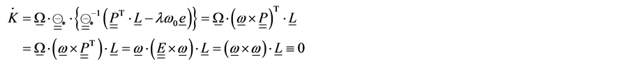
We proved that K-const., hence from Equation (2.17) the energy integral has the following form

$\underset{\_}{\Omega }\cdot {\underset{\_}{\underset{\_}{\ominus }}}_{\ast }\cdot \underset{\_}{\Omega }=h\equiv \text{const}\text{.}$ (2.19)

3. Transformation of the Energy Integral

In general the turn-tensor can be expressed through three parameters. The energy integral gives a relation, which superposed on these parameters. Therefore, only two of them are independent variables, and the free rotations of the body are two-parameter movements.

Thus it’s necessary to find the general from of a two-parameter turn-tensor conserving the energy. The unit vector $\underset{\_}{m}$ may be introduced by

$\underset{\_}{m}={\underset{\_}{\underset{\_}{P}}}^{\text{T}}\cdot \widehat{\underset{\_}{L}},\left|\widehat{\underset{\_}{L}}\right|=1,\underset{\_}{m}\cdot \underset{\_}{m}=1$ (3.1)

Substituting Equations (2.16), (3.1) into equation (2.19), we have

$\left(\underset{\_}{m}-\frac{\lambda {\omega }_0}{l}\underset{\_}{e}\right)\cdot {\underset{\_}{\underset{\_}{\ominus }}}_{\ast }^{-1}\cdot \left(\underset{\_}{m}-\frac{\lambda {\omega }_0}{l}\underset{\_}{e}\right)=\frac{h}{l^2},\widehat{\underset{\_}{L}}=\frac{\underset{\_}{L}}{l}$ (3.2)

Using Zhilin’s theorem [9] to represent the turn-tensor $\underset{\_}{\underset{\_}{P}}$ . The theorem of representation of the turn-tensor can be formulated: Let there be given two arbitrary unit vectors $\underset{\_}{\hat{u}}$ and $\underset{\_}{\hat{v}}$ . Any turn-tensor can be represented in the form composition of turns around vectors #Math_75# ,#Math_76# and $\widehat{\underset{\_}{\omega }}$

$\underset{\_}{\underset{\_}{P}}\left(t\right)=\underset{\_}{\underset{\_}{Q}}\left(\psi \left(t\right)\underset{\_}{\hat{u}}\right)\cdot \underset{\_}{\underset{\_}{Q}}\left(\theta \left(t\right)\widehat{\underset{\_}{\omega }}\right)\cdot \underset{\_}{\underset{\_}{Q}}\left(\phi \left(t\right)\underset{\_}{\hat{v}}\right);\widehat{\underset{\_}{\omega }}=\frac{\underset{\_}{\hat{u}}\times \underset{\_}{\hat{v}}}{\left|\underset{\_}{\hat{u}}\times \underset{\_}{\hat{v}}\right|}$ (3.3)

where $\psi \left(t\right),\phi \left(t\right)\text{and}\theta \left(t\right)$ are called angles of precession, nutation, and own rotation, respectively.

The success of solution depends on the appropriate of representation of the turn-tensor i.e. the equation of solution will be in complicated from with the unsuccessful choice of vectors $\underset{\_}{\hat{u}}$ and $\underset{\_}{\hat{v}}$ . Moreover, the unsuccessful choice of vectors $\underset{\_}{\hat{u}}$ and $\underset{\_}{\hat{v}}$ may lead to appearance of singular points in the solution. For choosing $\underset{\_}{\hat{u}}$ and $\underset{\_}{\hat{v}}$ we will use the fact: ${\underset{\_}{\underset{\_}{P}}}^{\text{T}}$ gives the motion of the kinetic moment with respect to the carrier body (see Formula (3.1)) and energy integral (3.2), which determine the path of the motion of vector of the kinetic moment with respect to the carrier body. Substituting (3.3) into (3.1), we get

$\underset{\_}{m}={\underset{\_}{\underset{\_}{Q}}}^{\text{T}}\left(\phi \underset{\_}{\hat{v}}\right)\cdot {\underset{\_}{\underset{\_}{Q}}}^{\text{T}}\left(\theta \widehat{\underset{\_}{\omega }}\right)\cdot {\underset{\_}{\underset{\_}{Q}}}^{\text{T}}\left(\psi \underset{\_}{\hat{u}}\right)\cdot \widehat{\underset{\_}{L}}$ (3.4)

It’s obvious, that $\underset{\_}{\hat{u}}=\widehat{\underset{\_}{L}}$ is a good choice, then

$\underset{\_}{m}={\underset{\_}{\underset{\_}{Q}}}^{\text{T}}\left(\phi \underset{\_}{\hat{v}}\right)\cdot {\underset{\_}{\underset{\_}{Q}}}^{\text{T}}\left(\theta \widehat{\underset{\_}{\omega }}\right)\cdot \widehat{\underset{\_}{L}}$ (3.5)

Since ${\underset{\_}{\underset{\_}{\ominus }}}_{\ast }$ is a symmetrical tensor, it may be represented as

${\underset{\_}{\underset{\_}{\ominus }}}_{\ast }={\theta }_1{\underset{\_}{d}}_1\otimes {\underset{\_}{d}}_1+{\theta }_2{\underset{\_}{d}}_2\otimes {\underset{\_}{d}}_2+{\theta }_3{\underset{\_}{d}}_3\otimes {\underset{\_}{d}}_3$ (3.6)

where ${\underset{\_}{d}}_1$ , ${\underset{\_}{d}}_2$ , ${\underset{\_}{d}}_3$ are unit vectors, which depend on this tensor. Then we can write

${\underset{\_}{\underset{\_}{\ominus }}}_{\ast }^{-1}=\frac{1}{{\theta }_1}{\underset{\_}{d}}_1\otimes {\underset{\_}{d}}_1+\frac{1}{{\theta }_2}{\underset{\_}{d}}_2\otimes {\underset{\_}{d}}_2+\frac{1}{{\theta }_3}{\underset{\_}{d}}_3\otimes {\underset{\_}{d}}_3$ (3.7)

The vectors $\underset{\_}{m}$ and $\underset{\_}{e}$ can be represented as

$\underset{\_}{m}=x_m{\underset{\_}{d}}_1+y_m{\underset{\_}{d}}_2+z_m{\underset{\_}{d}}_3$ (3.8)

$\underset{\_}{e}=e_1{\underset{\_}{d}}_1+e_2{\underset{\_}{d}}_2+e_m{\underset{\_}{d}}_3$ (3.9)

The choice of the vector $\underset{\_}{\hat{v}}$ is not unknown. This choice may be ${\underset{\_}{d}}_1$ , ${\underset{\_}{d}}_2$ , ${\underset{\_}{d}}_3$ or other vector. The solution does not contain singular points, if following inequality is valid.

$\forall t0\le \underset{\_}{m}\left(t\right)\cdot \underset{\_}{\hat{v}}<1$ (3.10)

i.e. the angle $\left(\alpha -\theta \right)$ belongs to $\left[0,\frac{\text{π}}{2}\right)$ , where the angle $\alpha$ is the angle between $\underset{\_}{\hat{v}}$ and $\widehat{\underset{\_}{L}}$ .

4. The Exact Solution in Particular Cases

Case (1): when ${\theta }_1={\theta }_2={\theta }_3$

In this case Equation (3.2) is reduced to:

$\underset{\_}{e}\cdot \underset{\_}{m}=\frac{1}{2\lambda l{\omega }_0}\left(l^2+{\lambda }^2{\omega }_0^2-h{\theta }_1\right)$ (4.1)

The intersection of the plane Equation (4.1) with the unit sphere $\left(\underset{\_}{m}\cdot \underset{\_}{m}=1\right)$ gives a hodograph of vector $\underset{\_}{m}$ . This hodograph is a circle, as shown in Figure 2.

Since vector $\underset{\_}{e}$ is perpendicular to the plane of hodograph, then it is suitable to represent the turn tensor of the carrier body $\underset{\_}{\underset{\_}{P}}$ in the form:

$\underset{\_}{\underset{\_}{P}}=\underset{\_}{\underset{\_}{Q}}\left(\psi \widehat{\underset{\_}{L}}\right)\cdot \underset{\_}{\underset{\_}{Q}}\left(\phi \underset{\_}{e}\right)$ (4.2)

The corresponding angular velocity of $\underset{\_}{\underset{\_}{P}}$ :

$\underset{\_}{\omega }=\stackrel{\dot{}}{\psi }\widehat{\underset{\_}{L}}+\underset{\_}{\underset{\_}{Q}}\left(\psi \widehat{\underset{\_}{L}}\right)\cdot \stackrel{\dot{}}{\phi }\underset{\_}{e}$ (4.3)

The right angular velocity is given by:

Figure 2. Hodograph of $\underset{\_}{m}$ .

$\underset{\_}{\Omega }={\underset{\_}{\underset{\_}{P}}}^{\text{T}}\cdot \underset{\_}{\omega }$ (4.4)

Substituting (4.3), (4.4) into equation (2.16) to get:

${\underset{\_}{\underset{\_}{\ominus }}}_{\ast }^{-1}\cdot \left\{l\underset{\_}{m}-\lambda {\omega }_o\underset{\_}{e}\right\}=\stackrel{\dot{}}{\psi }\underset{\_}{m}+\stackrel{\dot{}}{\phi }\underset{\_}{e}$ (4.5)

Hint

${\underset{\_}{\underset{\_}{\ominus }}}_{\ast }^{-1}=\frac{1}{{\theta }_1}\underset{\_}{\underset{\_}{E}}$ (4.6)

Rewriting Equation (4.5) as:

$\left(\stackrel{\dot{}}{\psi }-\frac{1}{{\theta }_1}\right)\underset{\_}{m}+\left(\stackrel{\dot{}}{\phi }+\frac{\lambda {\omega }_o}{{\theta }_1}\right)\underset{\_}{e}=0$ (4.7)

From the vectorial Equation (4.7) it follows that:

$\{\begin{array}{l}\stackrel{\dot{}}{\psi }=\frac{1}{{\theta }_1}\hfill \\ \stackrel{\dot{}}{\phi }=\frac{\lambda {\omega }_o}{{\theta }_1}\hfill \end{array}$ (4.8)

Then:

$\{\begin{array}{l}\psi =\frac{1}{{\theta }_1}t+{\psi }_o\hfill \\ \phi =\frac{\lambda {\omega }_o}{{\theta }_1}t+{\phi }_o\hfill \end{array}$ (4.9)

Equations (4.2), (4.3), (4.4), (4.9) and from $\stackrel{\dot{}}{\beta }$ which given in (2.16), give the exact solution of the problem.

Case (2): when ${\theta }_1={\theta }_2\ne {\theta }_3,\underset{\_}{e}={\underset{\_}{d}}_3$

Equation (3.2) may be represented in the following form:

$\frac{1}{{\theta }_1}\left(x_m^2+y_m^2\right)+\frac{1}{{\theta }_1}{z}_m^2-\frac{2\lambda {\omega }_o}{l{\theta }_3}{z}_m=\frac{h}{l^2}-\frac{{\lambda }^2{\omega }_o^2}{l^2{\theta }_3}$ (4.10)

Inserting (3.1) into (4.10), we get:

$A{z}_m^2-2B{z}_m+C=0$ (4.11)

where $A=\left(\frac{1}{{\theta }_3}-\frac{1}{{\theta }_1}\right),B=\frac{\lambda {\omega }_o}{l{\theta }_3},C=\frac{1}{{\theta }_3}+\frac{1}{{\theta }_1}+\frac{1}{l^2}.$

Then

$z_m=\frac{B\pm \sqrt{B^2-AC}}{A}$ (4.12)

The intersection of plane (4.12) with the unit Sphere $\left(\underset{\_}{m}\cdot \underset{\_}{m}=1\right)$ gives a hodograph of the vector $\underset{\_}{m}$ as shown in Figure 3.

Since:

$\underset{\_}{\underset{\_}{P}}=\underset{\_}{\underset{\_}{Q}}\left(\psi \widehat{\underset{\_}{L}}\right)\cdot \underset{\_}{\underset{\_}{Q}}\left(\phi {\underset{\_}{d}}_3\right)$

$\underset{\_}{\omega }=\stackrel{\dot{}}{\psi }\widehat{\underset{\_}{L}}+\stackrel{\dot{}}{\phi }\underset{\_}{\underset{\_}{Q}}\left(\psi \widehat{\underset{\_}{L}}\right)\cdot {\underset{\_}{d}}_3$

Figure 3. A horizontal hodograph of $\underset{\_}{m}$ .

$\underset{\_}{\Omega }=\stackrel{\dot{}}{\psi }\underset{\_}{m}+\stackrel{\dot{}}{\phi }{\underset{\_}{d}}_3$

Then:

${\underset{\_}{\underset{\_}{\ominus }}}_{\ast }^{-1}\cdot \left\{l\underset{\_}{m}-\lambda {\omega }_o\underset{\_}{e}\right\}=\stackrel{\dot{}}{\psi }\underset{\_}{m}+\stackrel{\dot{}}{\phi }{\underset{\_}{d}}_3$ (4.13)

where

$\{\begin{array}{c}\begin{array}{l}{\underset{\_}{\underset{\_}{\ominus }}}_{\ast }={\theta }_1\left(\underset{\_}{\underset{\_}{E}}-{\underset{\_}{d}}_3\otimes {\underset{\_}{d}}_3\right)+{\theta }_3{\underset{\_}{d}}_3\otimes {\underset{\_}{d}}_3,\hfill \\ \underset{\_}{e}={\underset{\_}{d}}_3,\underset{\_}{m}=x_m{\underset{\_}{d}}_1+y_m{\underset{\_}{d}}_2+z_m{\underset{\_}{d}}_3\hfill \end{array}\end{array}$ (4.14)

Substituting (4.14) into (4.13) to get:

$\{\begin{array}{l}\stackrel{\dot{}}{\psi }=\frac{1}{{\theta }_1},\hfill \\ \stackrel{\dot{}}{\phi }=l{z}_m-\lambda {\omega }_o-\frac{{\theta }_3}{{\theta }_2}{z}_m\hfill \end{array}$ (4.15)

$\{\begin{array}{l}\psi =\left(\frac{1}{{\theta }_1}\right)t+{\psi }_o,\hfill \\ \phi =\left(l{z}_m-\lambda {\omega }_o-\frac{{\theta }_3}{{\theta }_2}{z}_m\right)t+{\phi }_o\hfill \end{array}$ (4.16)

5. System of Differential Equations Describing the Rotation

Putting $\hat{v}={\underset{\_}{d}}_3$ in Equation (3.3) and by using $\underset{\_}{\Omega }={\underset{\_}{\underset{\_}{P}}}^{\text{T}}\cdot \underset{\_}{\omega }$ , we can drive

$\underset{\_}{\Omega }=\stackrel{\dot{}}{\phi }\cdot {\underset{\_}{d}}_3+\frac{\stackrel{\dot{}}{\theta }}{\sin \left(\alpha -\theta \right)}{\underset{\_}{d}}_3\times \underset{\_}{m}+\stackrel{\dot{}}{\psi }\underset{\_}{m}$ (5.1)

Substituting Equations (2.16), (3.1) into (5.1), we get

$\stackrel{\dot{}}{\Phi }{\underset{\_}{d}}_3+\frac{\stackrel{\dot{}}{\Theta }}{\sin \Theta }{\underset{\_}{d}}_3\times \underset{\_}{m}=\stackrel{\dot{}}{\psi }\underset{\_}{m}-l{\theta }_{\ast }^{-1}\cdot \underset{\_}{m}+\lambda {\omega }_0{\theta }_{\ast }^{-1}\cdot \underset{\_}{e}$ (5.2)

where $\Phi =\xi –\phi$ , $\Theta =\alpha -\theta \text{and}\widehat{\underset{\_}{L}}=\sin \alpha \cos \xi {\underset{\_}{d}}_2+\cos \alpha {\underset{\_}{d}}_3$

By using Equations (3.2), and (5.2). It is can be written

$\stackrel{\dot{}}{\psi }=\lambda {\omega }_0\underset{\_}{e}{\theta }_{\ast }^{-1}\cdot \underset{\_}{m}+\stackrel{\dot{}}{\Phi }{\underset{\_}{d}}_3\cdot \underset{\_}{m}+\frac{h}{l}-\frac{{\lambda }^2{\omega }_0^2}{l}\underset{\_}{e}\cdot {\theta }_{\ast }^{-1}\cdot \underset{\_}{e}$ (5.3)

From the Equation (3.5), we have

$\underset{\_}{m}=\widehat{\underset{\_}{L}}\cdot \underset{\_}{\underset{\_}{Q}}\left(\theta \hat{\omega }\right)\cdot \underset{\_}{\underset{\_}{Q}}\left(\phi {\underset{\_}{d}}_3\right)=\frac{\sin \theta }{\sin \alpha }{\underset{\_}{d}}_3+\frac{\sin \left(\alpha -\theta \right)}{\sin \alpha }\widehat{\underset{\_}{L}}\cdot \underset{\_}{\underset{\_}{Q}}\left(\phi {\underset{\_}{d}}_3\right)$ ,

Then we can get

$\underset{\_}{m}=\sin \left(\Theta \right)\cos \left(\Phi \right){\underset{\_}{d}}_1+\sin \left(\Theta \right)\sin \left(\Phi \right){\underset{\_}{d}}_2+\cos \left(\Theta \right){\underset{\_}{d}}_3$ (5.4)

Multiplying Equation (5.2) by ${\underset{\_}{d}}_1$ scalar product, and using Equations (5.3), and (5.4) we get the system of first order non linear differential equation

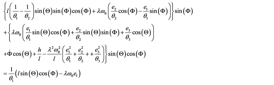(5.5)

Making use Equations (5.3), (5.4) and substituting them into Equation (5.2) after multiplying it by ${\underset{\_}{d}}_3\times \underset{\_}{m}$ scalar product. We can get

$\stackrel{\dot{}}{\Theta }=l\left(\frac{1}{{\theta }_1}-\frac{1}{{\theta }_2}\right)\sin \left(\Theta \right)\sin \left(\Phi \right)\cos \left(\Phi \right)+\lambda {\omega }_0\left(\frac{e_2}{{\theta }_2}\cos \left(\Phi \right)-\frac{e_1}{{\theta }_1}\sin \left(\Phi \right)\right)$ (5.6)

6. Numerical Solution

The system of Equations (5.5), (5.6) may be solved numerically under the necessary condition

$0\le \underset{\_}{m}\left(t\right)\cdot {\underset{\_}{d}}_3<1$ (6.1)

Considering this condition to avoid the singular points during calculations.

The common points of sphere (3.1) with the horizontal plane $z_m=0$ give a circle:

$x^2+y^2=1$ (6.2)

The intersection of surface (3.2) with $z_m=0$ is given by the equation of ellipse:

$M\left(x,y\right)={\left(\frac{x-x_0}{a}\right)}^2+{\left(\frac{y-y_0}{b}\right)}^2-1=0;$ (6.3)

$a=\frac{\sqrt{s_3}}{\sqrt{\frac{1}{{\theta }_1}-\frac{1}{{\theta }_3}}},b=\frac{\sqrt{s_3}}{\sqrt{\frac{1}{{\theta }_2}-\frac{1}{{\theta }_3}}},x_0=\frac{\lambda {\omega }_0{e}_1{\theta }_3}{l\left({\theta }_3-{\theta }_1\right)},y_0=\frac{\lambda {\omega }_0{e}_2{\theta }_3}{l\left({\theta }_3-{\theta }_2\right)}$

where $s_3=\frac{h}{l^2}-\frac{1}{{\theta }_3}+\frac{{\lambda }^2{\omega }_0^2}{l^2}\left(\frac{e_1^2}{{\theta }_3-{\theta }_1}+\frac{e_2^2}{{\theta }_3-{\theta }_2}+\frac{e_3^2}{{\theta }_3}\right)$ .

The distance between the origin and a point on the ellipse (6.3) may given by

$r\left(x,y\right)=\sqrt{x^2+y^2}$ (6.4)

To get the minimum and maximum distance between the origin and a point on the ellipse (6.3) the following steps may be done. Suppose them are $r_{\min }={\sigma }_z$ and $r_{\max }={\delta }_z$ . Solving the system:

$\{\begin{array}{l}\frac{\frac{\partial M}{\partial x}}{\frac{\partial r}{\partial x}}=\frac{\frac{\partial M}{\partial y}}{\frac{\partial r}{\partial y}},\hfill \\ M\left(x,y\right)=0\hfill \end{array}$ (6.5)

Four points are verifying the solution of the previous system (6.5). At these points $r\left(x,y\right)$ may be evaluated. The smallest real value of them is ${\sigma }_z$ and the largest real value is ${\delta }_z$ . If ${\sigma }_z,{\delta }_z<1$ or ${\sigma }_z,{\delta }_z>1$ valid, then the condition:

$0\le \underset{\_}{m}\left(t\right)\cdot {\underset{\_}{d}}_3<1$

will be satisfied. It is easy to see that the conditions

$\left({\sigma }_z,{\delta }_z<1\text{or}{\sigma }_z,{\delta }_z>1\right)$ (6.6)

are verifiable in Figure 4(a) and Figure 5(a) shows the intersection between the surface (6.3) and sphere (6.2), Figure 4(b) and Figure 5(b) gives the intersection of (6.3), (6.2) with $z_m=0$ .

(a) (b) (c) (d)

Figure 4. (a) Intersection between the surface (6.3) and sphere (6.2); (b) Intersection of (6.3), (6.2) with $z_m=0$ ; (c) Oscillating nature of Θ; (d) Monotonically variation of Φ.

(a) (b) (c) (d)

Figure 5. (a) Intersection between the surface (6.3) and sphere (6.2); (b) Intersection of (6.3), (6.2) with $z_m=0$ ; (c) Oscillating nature of Θ; (d) Oscillating nature of Φ.

7. Discussion and Conclusion

To understand and predict the behaviour of gyrostat it is necessary to know the suitable form of the turn-tensor of the carrier body,

$\begin{array}{l}\underset{\_}{\underset{\_}{P}}\left(t\right)=\underset{\_}{\underset{\_}{Q}}\left(\psi \left(t\right)\widehat{\underset{\_}{L}}\right)\cdot \underset{\_}{\underset{\_}{Q}}\left(\theta \left(t\right){\widehat{\underset{\_}{\omega }}}_i\right)\cdot \underset{\_}{\underset{\_}{Q}}\left(\phi \left(t\right){\underset{\_}{d}}_i\right),{\widehat{\underset{\_}{\omega }}}_i=\frac{\underset{\_}{L}\times {\underset{\_}{d}}_i}{\left|\underset{\_}{L}\times {\underset{\_}{d}}_i\right|};\\ \text{if}\left({\sigma }_i<1,{\delta }_i<1\right)\text{or}\left({\sigma }_i>1,{\delta }_i>1\right)\end{array}$ (7.1)

The angle precession $\psi$ is varying monotonically but the variation of angle of nutation $\theta$ has oscillating nature. The angle of own rotation $\phi$ is varying monotonically if the unit vector ${\underset{\_}{d}}_i$ will be inside the hodograph of the vector $\underset{\_}{m}$ , but if it will be outside this hodograph, then the variation of angle $\phi$ has an oscillating nature. The turn-tensor $\underset{\_}{\underset{\_}{P}}\left(t\right)$ may be represented by another vector except ${\underset{\_}{d}}_i\left(i=1,2,3\right)$ when the condition $\left({\sigma }_i<1,{\delta }_i<1\right)$ or $\left({\sigma }_i>1,{\delta }_i>1\right)$ is invalid. Particularly, the exact solution is found when $\left({\theta }_1={\theta }_2={\theta }_3\right)$ and when $\left({\theta }_1={\theta }_2\ne {\theta }_3,\underset{\_}{e}={\underset{\_}{d}}_3\right)$ . Excluding the singular points under the conditions $\left({\sigma }_i<1,{\delta }_i<1\right)$ or $\left({\sigma }_i>1,{\delta }_i>1\right)$ the numerical solution is represented graphically for some given parameters.

Conflicts of Interest

The authors declare no conflicts of interest.

References

[1]	Galal, A.A. (2001) Free Rotation of One-Rotor Gyrostat. APM, Saint-Petersburg (Repino), 263-271.
[2]	Grammel, R. (1950) Der Kreisel Seine Theorie und Anwendungen. Berlin-Gottingen Heidelberg, Springer. https://doi.org/10.1007/978-3-662-30589-8
[3]	Lyudmila, M.K. (1972) New Cases of Integrability of Equation of the Motion of Gyrostat. Ph.D. Thesis, St. Petersburg State Technical University, St. Petersburg, 53-69. (In Russian)
[4]	Magnus, K. (1971) Der Kreisel, Theorie und Anwendungen. Springer-Verlag Berli-Heidelberg. New York, Course and Lectures, No. 53, 1-144.
[5]	Lurie, A.I. (1961) Analytical Mechanics. Nauka, Moscow. (In Russian)
[6]	Savet, P.H. (1961) Gyroscopes, Theory and Design. McGraw-Hill, New York.
[7]	Smolnikov, B.A. and Stepanova, M.V. (1981) Free Permanent Rotations of Gyrostat. Mechanics of Rigid Body. No. 3, 121-196. Academy of Sciences of USSR, Moscow. (In Russian)
[8]	Volterra, V. (1899) Sur la theorie des variations des latitudes. Acta Mathematica, 22, 201-358. https://doi.org/10.1007/BF02417877
[9]	Zhilin, P.A. (1996) A New Approach to the Analysis of Free Rotation of Rigid Bodies. Zeitschrift für Angewandte Mathematik und Mechanik, 76, 187-204. https://doi.org/10.1002/zamm.19960760402