Computational Approach to Control Laws of Strict-Feedback Nonlinear Systems ()

1. Introduction
Nonlinear system study has been advanced greatly in the last few decades. In particular, the back-stepping method was discovered and applied in the design of nonlinear control systems [1] .
The complexity of the computation involved in the study of nonlinear systems makes the use of computer algebra inevitable. In fact, the nature of the computation of back- stepping, a recursive procedure, is symbolic.
Computer Algebra System, also called CAS for symbolic computation, has been advanced greatly in the last few decades as well. Powerful computer algebra systems now are capable to do numerical computation, symbolic computation, graphing, and pro- gramming. The rich built-in functions in a computer algebra system make the study of complicated systems handy.
Computer algebra has been used in the study of nonlinear systems in general (for example, see [1] - [5] ), and in the study of back-stepping in particular (for example, see [6] ). However, for some reasons, computer algebra systems are not yet popular in the engineering society. In this paper, we show how computer algebra systems can be successfully used in computing a control law for strict-feedback systems.
The use of computer algebra systems allows researchers and students to save time from tedious and error prone computations and focus on the basic ideas and methods.
Therefore, it is not only important for industrial applications, but also for research and education. Maple is one of the most powerful computer algebra systems in the world. We use Maple to compute control laws of strict-feedback systems. We also use Maple to verify the stability and other behaviors of the systems.
In this paper, Maple procedures are listed and examples are given.
To familiarize the audience in the community of control systems with computer algebra systems is also a goal of this paper.
2. Back-Stepping for Strict-Feedback Systems
Assume a state vector , we define nonlinear recursive and strict-feedback systems by the following:
 (1)
(1)
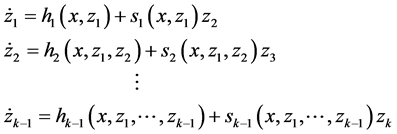 (2)
(2)
The recurrence relation (2) can be briefly described by:
 (3)
(3)
for , where
 , and n is the vector field dimension. The value
  is the plant input and the new state variable zk is considered the plant output.
The functions f and g in relation (1) can be described by
 ,
,  ,
, .
.
Lyapunov Stable Control Design:
Assume that for the system,  , there exists a continuously differentiable feedback control law
  a smooth, positive definite, and radially unbounded function
such that
a smooth, positive definite, and radially unbounded function
such that
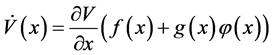
is negative definite, i.e., the system

is asymptotically stable.
The following recursive procedure is used to compute a control law to stabilize the above strict-feedback system [7] .

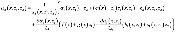
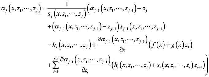
where ![]() The control law can be described:
The control law can be described:![]() .
.
There are other control laws based on back-stepping. The above control law may not be the best choice for a particular control system with particular design concerns. However The program can be modified if some application oriented guidelines are given.
This paper is not for the detailed discussion of the back-stepping method; instead, it is for the computation of the method. From the above formulas one can see that the computation is very tedious and time-consuming.
Computer algebra can be used to compute the control laws.
3. Maple Procedures
The following is a Maple Procedure for computing the control law
of nonlinear strict-feedback systems. The first argument of the procedure is![]() . The second argument of it is
. The second argument of it is![]() . The third and the fourth arguments are the known Lyapunov function,
. The third and the fourth arguments are the known Lyapunov function, ![]() , and the control law,
, and the control law, ![]() , for system
, for system![]() .
.
The following program is the Maple Procedure designed to solve the dynamical control systems in (1), (2), and (3), in generalto compute a control law to stabilize the strict-feedback system.
restart;
with(linalg);
strict:= proc (f, g, h, s, V, a)
local z, alpha, n, k, i, j;
with(linalg); n := vectdim(f); k := vectdim(s);
for i to 1 do
alpha[1] := simplify((-z[1]+a-add((diff(V, x[i]))*g[i], i = 1 .. n)-h[1]+(diff(a, x[1]))*(z[1]*g[1]+f[1]))/s[1]);
if k = 1 then break end if;
alpha[2] := simplify((alpha[1]-z[2]-(z[1]-a)*s[1]-h[2]+add((diff(alpha[1], x[i]))*(z[1]*g[i]+f[i]), i = 1 .. n)+(diff(alpha[1], z[1]))*(z[2]*s[1]+h[1]))/s[2]);
if k = 2 then break end if;
for j from 3 to k do
alpha[j] := simplify((alpha[j-1]-z[j]-(z[j-1]-alpha[j-2])*s[j-1]-h[j]+add ((diff(alpha[j-1], x[i]))*(z[1]*g[i]+f[i]), i = 1 .. n)+add((diff(alpha[j-1], z[i]))*(z[i+1]*s[i]+h[i]), i = 1 .. j-1))/s[j])
end do
end do
end proc;
Program (1): This table is a copy of the Maple procedure named “strict” that will be used to execute for a variety of Nonlinear Control Systems.
The following is the result of the execution of the Maple procedure to show phase portraits of second order nonlinear systems with arbitrary initial conditions. The arguments described in the above “strict” procedure are systems of equations and numbers of initial value problems (up to 20)
portrait:=proc(sys, m, tm, icr)
local r,n,s,sx,sxi1,i,x,y,a,b;
with(plots):
x:=op(1,lhs(sys[1])); y:=op(1,lhs(sys[2]));
n:=m; r:=rand(-5..5): s:=array(1..n): sx:=array(1..n): sxi1:=array(1..n):
for i from 1 to n do
s[i]:=dsolve({op(sys),subs(op(x)=0,x)=icr*(rand())/(2*10^(12))r(),subs(op(y)=0,y)=icr*(rand())/(2*10^(12))r()},{x,y},numeric);
od;
for i from 1 to 1 do
sx[1]:=t->rhs(s[1](t)[2]): sxi1[1]:=t->rhs(s[1](t)[3]):
if n=1 then break fi;sx[2]:=t->rhs(s[2](t)[2]): sxi1[2]:=t->rhs(s[2](t)[3]):
if n=2 then break fi;sx[3]:=t->rhs(s[3](t)[2]):sxi1[3]:=t->rhs(s[3](t)[3]):
if n=3 then break fi;sx[4]:=t->rhs(s[4](t)[2]):sxi1[4]:=t->rhs(s[4](t)[3]):
if n=4 then break fi;sx[5]:=t->rhs(s[5](t)[2]):sxi1[5]:=t->rhs(s[5](t)[3]):
if n=5 then break fi;sx[6]:=t->rhs(s[6](t)[2]): sxi1[6]:=t->rhs(s[6](t)[3]):
if n=6 then break fi;sx[7]:=t->rhs(s[7](t)[2]): sxi1[7]:=t->rhs(s[7](t)[3]):
if n=7 then break fi;sx[8]:=t->rhs(s[8](t)[2]):sxi1[8]:=t->rhs(s[8](t)[3]):
if n=8 then break fi;sx[9]:=t->rhs(s[9](t)[2]):sxi1[9]:=t->rhs(s[9](t)[3]):
if n=9 then break fi;sx[10]:=t->rhs(s[10](t)[2]):sxi1[10]:=t->rhs(s[10](t)[3]):
if n=10 then break fi;sx[11]:=t->rhs(s[11](t)[2]): sxi1[11]:=t->rhs(s[11](t)[3]):
if n=11 then break fi;sx[12]:=t->rhs(s[12](t)[2]): sxi1[12]:=t->rhs(s[12](t)[3]):
if n=12 then break fi;sx[13]:=t->rhs(s[13](t)[2]):sxi1[13]:=t->rhs(s[13](t)[3]):
if n=13 then break fi;sx[14]:=t->rhs(s[14](t)[2]):sxi1[14]:=t->rhs(s[14](t)[3]):
if n=14 then break fi;sx[15]:=t->rhs(s[15](t)[2]):sxi1[15]:=t->rhs(s[15](t)[3]):
if n=15 then break fi;sx[16]:=t->rhs(s[16](t)[2]): sxi1[16]:=t->rhs(s[16](t)[3]):
if n=16 then break fi;sx[17]:=t->rhs(s[17](t)[2]): sxi1[17]:=t->rhs(s[17](t)[3]):
if n=17 then break fi;sx[18]:=t->rhs(s[18](t)[2]):sxi1[18]:=t->rhs(s[18](t)[3]):
if n=18 then break fi;sx[19]:=t->rhs(s[19](t)[2]):sxi1[19]:=t->rhs(s[19](t)[3]):
if n=19 then break fi;sx[20]:=t->rhs(s[20](t)[2]):sxi1[20]:=t->rhs(s[20](t)[3]):
if n=20 then break fi;
od;
a:=plot([seq([sx[i],sxi1[i],0...001],i=1..n)],style=point,labels=[x, y],caption="The phase portrait with random initial conditions");
b:=plot([seq([sx[i],sxi1[i],0..tm],i=1..n)],labels=[x, y],caption="The phase portrait with random initial conditions"); print(display(a,b)); sx,sxi1:
end:
Program (2): This table represents the execution of the Maple procedure named “portrait” to produce a sequence of graphs (sgraph) for the strict-feedback nonlinear control systems.
Due to the paper size limitation, Maple procedure, and sgraphs to show the graphs of third order systems with arbitrary initial conditions are not listed. The arguments of the procedure are also systems of equations and numbers of initial value problems.
Examples
The following examples show that the above procedures work well.
Example 1: Given a dynamical system (see the reference [8] , pp. 592-594)
![]() (4)
(4)
The following are the Maple commands and results of the control solutions.
>![]()
![]()
![]()
>![]()
![]()
![]()
>![]()
![]()
![]()
>![]()
![]()
We use our Maple procedure “portrait” to demonstrate the phase portraits of the system with random initial conditions. It can be seen that the system is globally asymptotically stable. Since the procedure “portrait” uses different variable names and deeds for forming systems of differential equations in the Maple setting, we converted u to a suitable form first.
>![]()
![]()
>![]()
![]()
>![]()
The portrait in Figure 1 demonstrates the global stability of the strict feedback control systems with one level integrator z1 about the equilibrium point.
Now consider the nonlinear system (4) with two integrators z1 and z2.
![]() (5)
(5)
The following are the Maple commands and results.
![]()
Figure 1. Phase portrait of a nonlinear control system (4) with random initial conditions.
By executing the Maple procedure “strict” from the Program (1) and the “portrait” procedure from Program (2), we can generate a sequence of graphs that we labeled as a[1], a[2], and a[3].
>![]()
![]()
![]()
>![]()
![]()
>![]()
![]()
>![]()
![]()
>![]()
>![]()
![]()
![]() (Figure 2).
(Figure 2).
Example 2: The following example demonstrates three levels of integrators for back-stepping control (see the reference [9] , p. 35)
![]() (6)
(6)
We initiate functions f and g as necessary by (1). We use the Lyapunov function V to execute the Maple procedure “strict”.
![]() a[1]
a[1]![]() a[2]
a[2]![]() a[3]
a[3]
Figure 2. a[1], a[2]), and a[3] are phase portraits of the nonlinear control system (5) in two levels using back-stepping algorithm.
>![]()
![]()
![]()
>![]()
![]()
![]()
>![]()
![]()
![]()
>![]()
![]()
Example 3: The following example is a nonlinear control system selected from the reference ( [10] , pp. 633-634):
![]() (7)
(7)
We use functions f and g from the system (7) to be used for Equation (1). Running the Maple procedure “strict” from the Program (1) produces the solution. The “portrait” procedure generates a sequence of graphs that we labeled b[1], b[2], and b[3].
>![]()
![]()
![]()
>![]()
![]()
![]()
>![]()
![]()
![]()
>![]()
![]()
![]()
>![]()
![]()
![]()
>![]()
![]()
>![]()
![]()
>![]()
![]()
>![]()
>![]()
![]()
![]() (Figure 3)
(Figure 3)
4. Conclusions
This paper shows the advantages of computer algebra systems like Maple in computation of nonlinear systems. Maple is successfully used to compute back-stepping control laws of nonlinear strict-feedback systems. The stability of systems with computed control laws is also verified by Maple procedures. As demonstrated by other researchers, computer algebra can be used for computing control laws of other systems with back- stepping. In general, it can be used to solve computation problems in science and engineering.
![]() b[1]
b[1]![]() b[2]
b[2]![]() b[3]
b[3]
Figure 3. The “portrait” procedure generates a sequence of graphs b[1], b[2], and b[3] for phase portrait of nonlinear control system (7).
We hope that more researchers, engineers, and students will take advantage of computer algebra systems as a tool in problem solving. Computer algebra systems should play more important roles in industry, research, and education.