Received 15 May 2016; accepted 26 June 2016; published 29 June 2016

1. Introduction
Convertible bonds are complicated and broadly used financial instruments combining the characteristics of stocks and bonds. In recent years, convertible bond has become a new investment product for the investors. The possibility to convert the bond into a predetermined number of stocks offers the chance to participate in rising stock prices with limited loss, given that the issuer does not default on its bond obligation. Convertible bonds often contain other embedded options such as call and put provisions. These options can be specified in various different ways, which make the products more complex. Especially, conversion and call opportunities may occur in case of certain restricted time periods with given stock price conditions, which results in the changing of the call price with time. The study of the convertible bond has a long history, firstly appearing in 1843; however, the pricing theory is relatively backward. With the work of Black and Scholes (1973) [1] and Merton (1973) [2] on the option pricing theory (B-S formula), Ingersoll (1977) [3] and Brennan and Schwartz (1980) [4] were the first to apply the B-S formula in pricing the convertible bonds. Tsiveriotis and Fernandes (1998) [5] innovatively divided the convertible bonds into two parts including the stock option and the pure cash flow. Davis and Lischka (1999) [6] considered the price of convertible bonds affected by the default risk, and a more complex three- factor model was proposed. Li (2008) [7] derived the stochastic interest rate model for the Vasicek model and the CIR model of the convertible bond pricing formula; the simulation results show that the results of the CIR model in the market are more reasonable than those by using the Vasicek model. In the pricing of convertible bonds, the most widely used numerical pricing methods include tree graph method (such as the Binomial tree model and triple tree model), finite difference method, finite element method, Monte Carlo method [8] - [16] and so on.
The purpose of this paper is to study the pricing of convertible bonds with call provision. By using the method for option pricing, the closed form of the price for convertible bond is presented.
The paper is organized as follows. In Section 2, we introduce the content of convertible bond with call provision briefly, and establish the pricing model for the convertible bonds with call provision. In Section 3, we solve the partial differential equation established for the convertible bonds, and give the closed form solution. Section 4 is a conclusion.
2. Convertible Bond with the Call Provision
Convertible bond has the characteristics of the implied stock option, the convertible bond holder once decided to execute the options, it becomes the shareholders of the company, and the right has no difference to the original company shareholder. The main impact for the holders to convert or not is the underlying asset price, the bond holders often choose to continuously hold or immediately convert into shares of the company based on the stock prices, when stock prices continued to slump or located in a special given regime, the bonds holder always held in hand to the maturity time or directly sell it to other investors; when stock prices continue to rise or the conversion is profitable, the holders usually choose convert the bonds into shares, and the amount of the trading profits depends of the specific stock price in the market.
However, there is possible that its stock price in the market continues to rise, its converted value far exceeds the profit obtained by holding to the maturity, which, to some extent, has serious impact on the interests of the previously-existing shareholders of the company. Therefore, the benefit issuers can reduce their cost of the issuance through establishing the call provision, to avoid the loss due to stock price soaring and market interest rates. The call provisioncan accelerate the conversion process and relieve the company’s financial pressure. Redemption usually occurs in case that the stock market price is far higher than the conversion price. When the company announces the redemption, bond holders usually immediately opted conversion to avoid loss.
Here, we employ a standard assumption that the stock price movement St meet geometric Brownian motion,

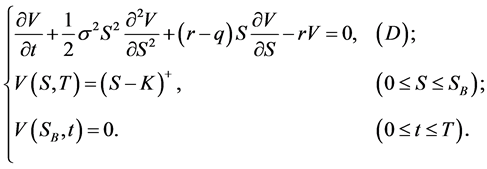
where μ is expect return rate (constant), σ is the volatility of the stock price, dWt is standard Brownian motion. Since the value of convertible bonds is related to the stock price and time, we use  to represent convertible bonds value with call provision. When the stock price of the company rises to the barrier fixed in advance (S = SB), the issuer announced the redemption of bonds. At this point, investors immediately implement the contract to convert the convertible bonds into stocks in order to obtain a higher interest. If one chooses to continue to hold the bond, he will get the bond value. When the stock price S reaches barrier value SB, the convertible bond will be executed. Let D a solution area as follows
 (1.1)
(1.1)
Then the final revenue function of the convertible bonds value is
 (1.2)
(1.2)
where ST is stock price at maturity date, K is transforming shares price stipulated in the contract, SB is stock price redemptive threshold stipulated by the issuer. Here  is the indicator function of ω (abbreviated as
 ),
),
 (1.3)
(1.3)
Clearly,  The termination conditions on t = T is
 (1.4)
(1.4)
In the given region  by using the classical method [17] , Black-Scholes equation for the convertible bonds value is
 (1.5)
(1.5)
To sum up, the pricing of convertible bonds with call provision is a specific boundary value problem for the Black-Scholes equation, which has similar properties of the up-and-out options to some extent. Compared with the standard options, it has more boundary conditions.
3. Pricing Model and Its Solution
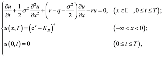
The pricing process of convertible bonds is, in the area , to solve the partial differential equation
 (1.6)
(1.6)
Make the transformation
 (1.7)
(1.7)
Then
 (1.8)
(1.8)
where ![]()
Define
![]() (1.9)
(1.9)
with
![]() (1.10)
(1.10)
![]() (1.11)
(1.11)
Based on (1.9), W is suitable for definite solution problems on the area![]() , we have
, we have
![]() (1.12)
(1.12)
By using the mirror methods, defining
![]() (1.13)
(1.13)
It is clearly![]() , that is,
, that is, ![]() is an odd-functions. Considering the Cauchy problem on the
is an odd-functions. Considering the Cauchy problem on the![]() , one gets
, one gets
![]() (1.14)
(1.14)
which is a odd function. The limitations on ![]() will be suitable for solution of the problem (1.12).
will be suitable for solution of the problem (1.12).
The solution of Cauchy problem (1.14) can be expressed as the Poisson equation
![]()
Then
![]() (1.15)
(1.15)
From (1.9), inserting ![]() into
into ![]() shows
shows
![]()
where
![]()
then
![]()
![]()
![]()
and
![]()
then
![]()
This, together (1.7), yields
![]() (1.16)
(1.16)
with
![]()
4. Conclusions
In this paper, based on the analysis of the execution conditions of convertible bonds with call provision, by solving a certain boundary value problem of the Black-Scholes equation, the closed form of the pricing formula is obtained.
In reality, the holders of convertible bonds tend to be risk-averse; owners generally hold the convertible bonds until the maturity date to obtain the bond interest as income, but when stock prices rise to a certain level (as defined for redemption), in order to obtain more profits, the holder will convert the bonds to the related stock, and sell the stocks in the secondary market. This paper just provides a theoretical evaluation of the bond for the investors. In this sense, the studied model in the paper is interesting and realistic.