Inverse Spectral Theory for a Singular Sturm Liouville Operator with Coulomb Potential

Etibar S. Panakhov^1*, Ismail Ulusoy²

¹Department of Mathematics, Firat University, Elazig, Turkey.
²Department of Mathematics, Adiyaman University, Adiyaman, Turkey.

DOI: 10.4236/apm.2016.61005                

Abstract

We consider the inverse spectral problem for a singular Sturm-Liouville operator with Coulomb potential. In this paper, we give an asymptotic formula and some properties for this problem by using methods of Trubowitz and Poschel.

Keywords

Coulomb Potential, Asymptotic Formula, Normalizing Eigenfunction

Received 21 September 2015; accepted 18 January 2016; published 21 January 2016

1. Introduction

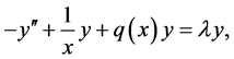
The Sturm-Liouville equation is a second order linear ordinary differential equation of the form

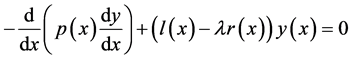(1.1)

for some 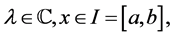and. It was first introduced in an 1837 publication [1] by the eminent French mathematicians Joseph Liouville and Jacques Charles François Sturm. The Sturm-Liouville Equation (1.1) can easily be reduced to form

(1.2)

If we assume that p(x) has a continuous first derivative, and p(x), r(x) have a continuous second derivative, then by means of the substitutions

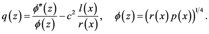
where c is given by

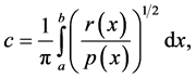
Equation (1.1) assumes the form (1.2) replaced by; where

The transformation of the general second order equation to canonical form and the asymptotic formulas for the eigenvalues and eigenfunctions was given by Liouville. A deep study of the distribution of the zeros of eigenfunctions was done by Sturm. Firstly, the formula for the distribution of the eigenvalues of the single dimensional Sturm operator defined in the whole of the straight-line axis with increasing potential in the infinity was given by Titchmarsh in 1946 [2] [3] . Titchmarsh also showed the distribution formula for the Schrödinger Operator. In later years, Levitan improved the Titchmarsh’s method and found important asymptotic formula for the eigenvalues of different differential operators [4] [5] . Sturm-Liouville problems with a singularity at zero have various versions. The best known case is the one studied by Amirov [6] [7] , in which the potential has a Coulomb-type singularity

at the origin. In these works, properties of spectral characteristic were studied for Sturm-Liouville operators with Coulomb potential, which have discontinuity conditions inside a finite interval. Panakhov and Sat estimated nodal points and nodal lengths for the Sturm-Liouville operators with Coulomb potential [8] -[10] . Basand Metin defined a fractional singular Sturm-Liouville operator having Coulomb potential of type A/x [11] .

Let’s give some fundamental physical properties of the Sturm-Liouville operator with Coulomb potential. Learning about the motion of electrons moving under the Coulomb potential is of significance in quantum theory. Solving these types of problems provides us with finding energy levels of not only hydrogen atom but

also single valance electron atoms such as sodium. For the Coulomb potential is given by, where r

is the radius of the nucleus, e is electronic charge. According to this, we use time-dependent Schrödinger equation

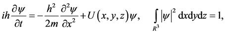
where is the wave function, h is Planck’s constant and m is the mass of electron.

In this equation, if the Fourier transform is applied

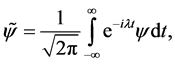
it will convert to energy equation dependent on the situation as follows:

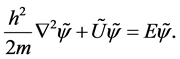
Therefore, energy equation in the field with Coulomb potential becomes

If this hydrogen atom is substituted to other potential area, then energy equation becomes

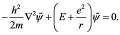
If we make the necessary transformation, then we can get a Sturm-Liouville equation with Coulomb potential

where is a parameter which corresponds to the energy [12] .

Our aim here is to find asymptotic formulas for singular Sturm-Liouville operatör with Coulomb potential with domain

~

Also, we give the normalizing eigenfunctions and spectral functions.

2. Basic Properties

We consider the singular Sturm-Liouville problem

(2.1)

where the function. Let us denote by the solution of (2.1) satisfying the initial condition

(2.2)

and by the solution of same equation, satisfying the initial condition

(2.3)

Lemma 1. The solution of problem (2.1) and (2.2) has the following form:

(2.4)

where.

Proof. Since satisfies Equation (2.1), we have

Integrating the first integral on the right side by parts twice and taking the conditions (2.2) into account, we find that

which is (2.4).

Lemma 2. The solution of problem (2.1) and (2.3) has the following form:

(2.5)

Proof. The proof is the same as that of Lemma 1.

Now we give some estimates of and which will be used later. For each fixed x in [0, 1] the map is an entire function on which is real-valued on [13] . Using the estimate

we get

Since and

we have

(2.6)

From (2.6) the inequality is easily checked

(2.7)

where c is uniform with respect to q on bounded sets in.

Lemma 3 (Counting Lemma). [13] Let and be an integer. Then has exactly N roots, counted with multiplicities, in the open half plane

and for each, exactly one simple root in the egg shaped region

There are no other roots.

From this Lemma there exists an integer N such that for every there is only one eigenvalue in Thus for every

(2.8)

can be chosen independent of q on bounded sets of. Following theorem [13] shows that the eigenvalues are the zeroes of the map and these zeroes are simple.

Theorem 1. If is Dirichlet eigenvalue of q in, then

In particular,. Thus, all roots of are simple.

Proof. The proof is similar as that of ([13] , Pöschel and Trubowitz).

3. Asymptotic Formula

We need the following lemma for proving the main result.

Lemma 4. For every f in,

(3.1)

and

. (3.2)

Proof. Firstly, we shall prove the relation (3.1)

(3.3)

By the Cauchy-Schwarz inequality, we get

.

Since f is in, the last two integrals are equal to

So (3.3) is equivalent to

.

Finally, we shall prove the relation (3.2)

This proves the lemma.

The main result of this article is the following theorem:

Theorem 2. For,

.

Proof of the Main Theorem. Since it must be. Because is a nontrivial solution of Equation (2.1) satisfying Dirichlet boundary conditions, we have

(3.4)

From (2.7) someone gets the inequality

(3.5)

From (3.5) integral in the equation of (3.4) takes the form

By using difference formulas for sine we have

From Lemma 4 we get

Thus, by using this inequality (3.4) can be written in the form

(3.6)

From (2.8) we conclude that

(3.7)

Since and, (3.7) is equivalent to

.

So we get

. (3.8)

From (2.8) we have

In this case, the theorem is proved.

From this theorem, the map

from q to its sequences of Dirichlet eigenvalues sends into S. Later, we need this map to characterize spectra which is equivalent to determining the image of.

4. Inverse Spectral Theory

To each eigenvalue we associate a unique eigenfunction normalized by

Let’s define the normalizing eigenfunction:

Lemma 5. For,

This estimate holds uniformly on bounded subsets of.

Proof. Let and. By the basic estimate for,

By using this estimate we have

So we get

Thus we conclude that

Dividing by we get

.

Also, we need to have asymptotic estimates of the squares of the eigenfunctions and products

Lemma 6. For,

This estimate holds uniformly on bounded subsets of.

Proof. We know that

By the basic estimate for, we have

Hence,

Let

.

The map is real analytic on. Now we give asymptotic behavior for.

Theorem 3. Each is a compact, real analytic function on with

(4.1)

Its gradient is

(4.2)

The error terms are uniform on bounded subsets of.

Proof. From [14] we have

So we calculate the integral

Finally, since, we get

(4.3)

By the Cauchy-Schwarz inequality, we prove the theorem.

Let

Formula (4.3) shows that belongs to. By Theorem 3, the map

from q to its sequences of -values maps into the. So we obtain a map

from into the.

Theorem 4. [13] is one-to-one on.

Let be the Frechet derivative of the map at q.

Theorem 5. [14] is an isomorphism from onto.

Conflicts of Interest

The authors declare no conflicts of interest.

References

[1]	Sturm, C. and Liouville, J. (1837) Extrait d.un m emoire sur le d eveloppement des fonctions en series dont les di erents terms sont assujettis a satisfaire a une m eme equation di er entielle lin eaire, contenant un param etre variable. Journal de Math ematiques Pures et Appliqu ees. Journal de Mathématiques Pures et Appliquées, 2, 220-233.
[2]	Birkhoff, G.D. (1908) Boundary Value and Expansion Problems of Ordinary Linear Differential Equations. Transactions of the American Mathematical Society, 9, 219-231. http://dx.doi.org/10.1090/S0002-9947-1908-1500810-1
[3]	Titchmarsh, E.C. (1946) Eigenfunction Expansions Associated with Second-Order Differential Equations. Vol. 1, Clarendon Press, Oxford.
[4]	Titchmarsh, E.C. (1958) Eigenfunction Expansions Associated with Second-Order Differential Equations. Vol. 2, Clarendon Press, Oxford.
[5]	Levitan, B.M. (1978) On the Determination of the Sturm-Liouville Operator from One and Two Spectra. Mathematics of the USSR Izvestija, 12, 179-193. http://dx.doi.org/10.1070/IM1978v012n01ABEH001844
[6]	Amirov, R.Kh. (1985) Inverse Problem for the Sturm-Liouville Equation with Coulomb Singularity Its Spectra. Kand. Dissertasiya, Baku.
[7]	Topsakal, N. and Amirov, R. (2010) Inverse Problem for Sturm-Liouville Operators with Coulomb Potential Which Have Discontinuity Conditions inside an Interval. Mathematical Physics, Analysis and Geometry, 13, 29-46. http://dx.doi.org/10.1007/s11040-009-9066-y
[8]	Sat, M. and Panakhov, E.S. (2012) Inverse Nodal Problem for Sturm-Liouville Operators with Coulomb Potential. International Journal of Pure and Applied Mathematics, 80, 173-180.
[9]	Sat, M. and Panakhov, E.S. (2013) Reconstruction of Potential Function for Sturm-Liouville Operator with Coulomb Potential. Boundary Value Problems, 2013, Article 49.
[10]	Sat, M. (2014) Half Inverse Problem for the Sturm-Liouville Operator with Coulomb Potential. Applied Mathematics and Information Sciences, 8, 501-504. http://dx.doi.org/10.12785/amis/080207
[11]	Bas, E. and Metin, F. (2013) Fractional Singular Sturm-Liouville Operator for Coulomb Potential. Advances in Difference Equations, Article ID: 300. http://dx.doi.org/10.1186/1687-1847-2013-300
[12]	Blohincev, D.I. (1949) Foundations of Quantum Mechanics. GITTL, Moscow.
[13]	Poeschel, J. and Trubowitz, E. (1987) Inverse Spectral Theory. Academic Press, San Diego.
[14]	Guillot, J.-C. and Ralston, J.V. (1988) Inverse Spectral Theory for a Singular Sturm-Liouville Operatör on [0,1]. Journal of Differential Equations, 76, 353-373. http://dx.doi.org/10.1016/0022-0396(88)90080-0