Diffraction of a Plane Acoustic Wave from a Finite Soft (Rigid) Cone in Axial Irradiation

Dozyslav B. Kuryliak, Zinoviy T. Nazarchuk, Victor O. Lysechko

Department of Physical Basis for Diagnostic of Materials, Karpenko Physico-Mechanical Institute of the NAS of Ukraine, Lviv, Ukraine.

DOI: 10.4236/oja.2015.54015                

Abstract

The problem of diffraction of a plane acoustic wave by a finite soft (rigid) cone is investigated. This one is formulated as a mixed boundary value problem for the three-dimensional Helmholtz equation with Dirichlet (Neumann) boundary condition on the cone surface. The diffracted field is sought as expansion of unknown velocity potential in series of eigenfunctions for each region of the existence of sound pressure. The solution of the problem then is reduced to the infinite set of linear algebraic equations (ISLAE) of the first kind by means of mode matching technique and orthogonality properties of the Legendre functions. The main part of asymptotic of ISLAE matrix element determined for large indexes identifies the convolution type operator amenable to explicit inversion. This analytical treatment allows one to transform the initial diffraction problem into the ISLAE of the second kind that can be readily solved by the reduction method with desired accuracy depending on a number of truncation. All these determine the analytical regularization method for solution of wave diffraction problems for conical scatterers. The boundary transition to soft (rigid) disc is considered. The directivity factors, scattering cross sections, and far-field diffraction patterns are investigated in both soft and rigid cases whereas the main attention in the near-field is focused on the rigid case. The numerically obtained results are compared with those known for the disc.

Keywords

Acoustic Wave, Finite Cone, Disc, Far-Field Pattern, Scattering Cross Section, Near Field, Analytical Regularization Procedure

Received 19 November 2015; accepted 22 December 2015; published 25 December 2015

1. Introduction

A contemporary nondestructive testing and acoustic diagnostics of materials exploit the modelling simulation. The latter provides for interaction of waves with defects of canonical shapes for which some analytical and semi-analytical solutions of corresponding diffraction problems can be obtained. These solutions play a key role in benchmark data for common numerical methods. On the other hand, it is of importance to take into account physical characteristics of defects and constructions for obtained reliable results of diagnostics in a wide frequency range. It is clear that solutions of diffraction problems on impedance surface very often cannot be obtained in analytical forms. But one can obtain a solution by analytical method for soft and rigid surfaces which are the boundary cases of impedance. So here, we contemplate as a model of construction or defect a finite cone with these surfaces.

In the scientific literature, a significant number of works are devoted to the study of diffraction of acoustic waves in semi-infinite cones with different types of boundary conditions (Dirichlet, Neumann, impedance boundary condition). Infinite circular cones [1] -[7] are mainly considered. Diffraction elliptic cone is reviewed in [8] and one of limiting cases of the cone such as diffraction of acoustic waves on plane sectors is studied in [9] [10] . A semi-transparent cone is investigated in [11] . Scattering of electromagnetic wave by infinite cones is also considered (see, for example [12] ). It should be noticed that the infinite cone is explored from the mechanical point of view in [13] .

The Wiener-Hoрf method in combination with the method of Kontorovich-Lebedev integral transformations is used for the solution of the diffraction problem on finite hollow cones (where discs are considered as particular cases of cones) [14] [15] and on the semi-infinite cone formed by the finite and semi-infinite conical surfaces with different boundary conditions [16] . In publication [17] , the appropriate problem is solved on a finite cone with internal termination in one of the sectors. Analytical regularization procedure for diffraction problems on fragments of circular conical surfaces is proposed earlier in [18] [19] where an excellent survey of known results for diffraction by finite cone is done. This procedure is used for investigation of the finite cone [20] in the electromagnetic case. Geometrical theory of diffraction is used in [21] .

In this article, based on analytical regularization procedure [18] , we investigate a scattered field of a plane acoustic wave from the perfectly soft (rigid) finite cone in a different frequency range.

2. Statement of the Problem

Let us consider the perfectly soft (S) rigid (R) hollow finite cone 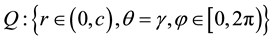(see Figure 1) in a spherical coordinate system. Cone is irradiated by a plane monochromatic acoustic wave that propagates along the symmetry of a cone in the direction with the velocity potential

, (1)

where is the vector, that defines a position of any point on the wave front, with the component ,; is the normal vector,; is the unit vector,; is a wave number, is the circular velocity, is the phase of the sound. Time factor is suppressed throughout this paper.

Since the velocity potential is symmetrical and independent of azimuth angle, than the scattering field is estimated in terms of the scalar (velocity) potential, satisfying the three-dimensional Helmholtz equation

, (2)

where is Laplace operator,

.

The unknown potential of the diffracted field is related to the sound pressure and to the velocity of particles by way of

, ,

and satisfies the Dirichlet (S) or Neumann (R) boundary conditions on the surface of the cone as follows:

for S; (3a)

Figure 1. Geometrical scheme of the problem.

for R. (3b)

Here is mean density; is the nabla operator.

In order to obtain the unique solution to the problem (2), (3), the additional conditions must be imposed on the unknown velocity potential: the radiation condition written as:

, ,

and the condition of the finiteness of energy in any bounded volume (edge condition) given as:

.

3. Solution of the Diffraction Problem

For solution of the diffraction problem let us decompose the space in regions

, , (4)

and determine the total field in the form of

Since the unknown scalar potential satisfies the Helmholtz Equation (2), we represent it by means of eigenfunctions in the appropriate domains as:

(5)

Here, , are unknown expansion coefficients; is the Legendre function; is the modified Bessel function; is the Macdonald function;; are positive roots of transcendental equations

, , for S; (6a)

, , for R, (6b)

where is the associated Legendre function, which is defined in [22] by the expression

.

For further convenience, in (5) we introduce with for S cone and with and the unknown for R cone.

The condition (6) guarantees satisfying the boundary condition at the conical surfaces for field presentation (5), as well as the finiteness of energy in the conical vertex. The Equation (5) satisfies the radiation condition at infinity.

We expand the scalar potential of an incident plane acoustic wave (1) in the series of spherical functions. Accounting a definition of indices for S and R cones leads to one

(7)

with for S and for R cases respectively;.

To find the unknown expansion coefficients in the (5), we use the mode matching technique

(8a)

(8b)

Substituting the relationship (5), (7) into Equation (8) leads to the series equations. In order to take into account the singularity of velocity of particles for, where is the distance to the edge in local coordinate system, we present these equations by way of

(9a)

(9b)

where the prime indicates the derivation with respect to the argument.

In order to reduce series Equation (9) to the infinite system of linear algebraic equations (ISLAE), we use a property of orthogonality of Legendre functions, which leads to [18]

. (10)

Here upper sign (“+”) corresponds to and lower sign (“?”) with and respectively; other notations are

, , for S; (11a)

, , for R. (11b)

First, we analyze the series Equation (9) for soft cone (S-case). For this purpose we substitute series (10) into Equation (9). Next, limiting the finite number of unknowns and excluding, we come to finite system of linear algebraic equations as follows:

; (12a)

, (12b)

where, , , , ,.

The main reason of this limitation is to provide the correct transition from Equation (12) to ISLAE (), the solution of which satisfies the Meixner condition at the conical edge. For this purpose, we introduce a growing sequence of roots, of transcendental Equation (6a) as:

. (13)

Next, in Equation (12) we pass to limit () and arrange the ISLAE according to sequence (13) as:

. (14)

Here; is the infinite matrix with the elements given as:

, (15)

where is the known vector

. (16)

Then we turn to analysis of rigid cone (R-case). To obtain the correct solution we take into account the values of pressure independent from in domains, which are determined by the unknowns, , , separately. This is done because the minimal (first) positive roots of the Equation (6b). Substituting (10) into (9) and limiting the finite number of the unknowns, we exclude, , () and come to ISLAE, where the first equation for indices looks as:

, (17)

and the others are determined by Equations (12a), (12b) with and respectively. Here.

According to our previous step for S-case, we introduce a growing sequence in the following:

. (18)

For this case we use the definition of roots of transcendental equations by way of (6b).

Further, passing to limit () and arranging (12) and (17) according to (18), we arrive at ISLAE in form of (14) with. Thus, it is easy to prove that for the other unknown.

4. Regularization of ISLAE

Taking into account the asymptotic properties of the modified Bessel and Macdonald functions for large indices, it is found that

(19)

which is correct for S and R cones.

Let us introduce the operator formed with the main parts of the asymptotic expression (15) as

, (20a)

and

. (20b)

Here

, ,

where is determined from the factorization of the even meromorphic function, which is regular in the strip with simple zeroes and poles at, that are located at the real axis out of the;

(21)

, are split functions, regular in the right and in the left half- planes respectively; and if in the regularity region, where upper sign corresponds to S and lower to R cones. Furthermore, the product of operators (20) represent the identity matrix I,.

Next, we formulate original diffraction problem (14) via the ISLAE of the second kind as follows:

. (22)

The technique described above is elaborated in [18] [19] and called the analytical regularization procedure.

ISLAE (22) admits the solution in the class of sequences with for S and for R cases. This fulfils all the necessary conditions for the existence of a unique solution of ISLAE (22), including the Meixner condition on the edge [18] .

We represent the other unknown coefficient in both S and R cases through the solution (22) by way of

,

where; is Kronecker symbol; upper indexes in brackets correspond to region with and lower ones to region with; and, for S and R cases respectively.

4.1. Low-Frequency Solution

Let us rewrite the basic ISLAE (22) for both Dirichlet and Neumann cases by way of

, (23)

where.

We take into account the low frequency asymptotic (19) and estimate the terms in expression (16) as:

for. (24)

Neglecting the terms of order, we immediately derive the approximate solution (23) as:

. (25)

Let us introduce a contour integral

, (26)

where the circle with radius that envelopes the simple poles of the integrand at () and. The integrand (26) decays as, if, where for S and for R cases. Next, using the residual theorem, it is found that

. (27)

Substituting (20b) into (25) and taking into consideration the expression (27) we arrive at

. (28)

The expression (28) gives the approximate solution of the diffraction problem in low-frequency case as series of.

4.2. Transition from Finite Cone to Disc

Let us consider the particular case of the problem when cone opening angle and becomes the disc. For this case, it is found that indices and are determine as:

(29)

with.

Let us present the kernel function (21) in explicit form with split function as:

(30)

Then, the couple of the regularization operators (20) is simplified and looks as:

(31a)

(31b)

Summarizing the above results, we prove that the solution of the wave diffraction problem for soft and rigid disc is reduced to the ISLAE, which we obtain from (22), taking into account expressions (29)-(31).

5. Numerical Calculation

All characteristics of the scattered field are calculated by reduction of ISLAE (22). The order of reduction has been chosen from the condition with. Based on the solution we consider a far-field characteristics for soft and rigid cones and near-field characteristics for rigid cone as they are more practical in use.

5.1. Far-Field Characteristics of Soft and Rigid Cones

Let us express the far-field pattern as

, (32)

where for its physical matter determines the scattered field in region.

With the help of (32), we analyze a diffraction pattern for soft and rigid finite cones when the incident plane wave (7) illuminates the apex () directly and aperture (), particularly for and. The curves in Figure 2 show the far-field patterns for soft cone. From Figure 2(a) we can observe a formation of the main lobe of diffraction pattern in the direction of forward scattering (curve 1), while backscattering () radiation tends to zero. The side lobes are formed for observation angles. The main lobe essentially grows with increasing. We also observe a typical peak about, which corresponds to specular reflection (see curve 2) and the wide deep shadow region for, whereas the contribution of radiation can be neglected. In Figure 2(b), we can observe the far field patterns in the case of plane wave irradiation of the cone aperture (). As it is seen from the behavior of curve 1 (compared to curve 1 and 2 in Figure 2(a)), the magnitudes of field scattering in direction is almost the same and significant radiation is observed in the range of.

In order to obtain a profound knowledge of the scattering mechanism, we compare the scattering properties of soft and rigid finite cones. Figure 3 shows the far-field patterns scattered by the rigid cone with the same geometrical parameters as in the previous case. Comparison of the curves in Figure 2(a), Figure 2(b) and Figure 3(a), Figure 3(b) visually, we find the similar scattering properties for soft and rigid finite cones illuminated by the plane wave, which propagates along the conical axis. The main difference is the inherent backscatter effect for the sharp rigid cone and its lack for the same soft cone.

We verified our results by comparing them with those obtained for circular soft (rigid) disc when and. In Figure 4, the magnitudes of the velocity potential is plotted as a function of the polar angle. The solid curve 1 (3) is obtained by us for soft (rigid) disc, while the dashed ones 2 (4) are obtained in [6] . There is an excellent agreement for all values of.

Our further examination aims at studying the energy characteristics of scattering. First of all, we determine the directivity factor [23] as:

(a) (b)

Figure 2. Far-field patterns scattered by the soft cone for different wave parameter kc. (a); (b). Curve 1 corresponds to and curve 2 to.

(a) (b)

Figure 3. Far-field patterns scattered by the rigid cone for different wave parameters kc. (a); (b). Curve 1 corresponds to, curve 2 to.

(a) (b)

Figure 4. The angular dependence of far field pattern. (a) Soft disc; (b) Rigid disc. Full line 1 (2) gives our calculation, broken line 3 (4) the values acording to [6] .

. (33a)

Applying (32) for (33a) it is found that

. (33b)

In Figure 5(a), we can see the monotonous increase of the directivity factor for soft finite cone with the growth of wave parameter and cone-generating angle. In the case of a rigid cone (Figure 5(b)), the growth of is similar, however with oscillations. This indicates that the formation of far-field radiation in direction is not monotonuous. The maximum value is expected to be observed for wide cones (). For long wave (), we have about () for a soft (rigid) cone. The latter corresponds to the case of the pulsating (oscillating) disc. So we see that directivity factor can be improved only by increasing the wave parameter and cone-generating angle. Besides, one can obtain a good concentration of energy in forward direction.

Let us express the total scattering cross section [23] as:

. (34)

The scattering cross section as a function of the parameter for soft and rigid cones with different opening angles is shown in Figure 6(a), Figure 6(b) respectively.

The curves shown in Figure 6(a) have different origins and these are shown in Table 1. They indicate to better scattering properties of the soft structure than of the rigid one in low-frequency range (see Figure 6(b)). The further increase of curves come to almost constant value (Figure 6(a)). The behavior of the curves in Figure 6(b) shows the decay of their oscillations with the increase of, as well as the shift of the major peaks

(a) (b)

Figure 5. The series of the directivity factor. (a) Soft cone; (b) Rigid cone.

(a) (b)

Figure 6. The series of the scattering cross section. (a) Soft cone; (b) Rigid cone.

with the increase of to the low-frequency region. This is observed as a result of the well-known piston action in low-frequency range. Its lowest level is observed for cone-generating angle and wave parameter about, with the higher peaks for a wide cone, for instance, when, the wave parameter is.

5.2. Some Near-Field Characteristics

Let us derive the total field potential representation at the point located on the finite rigid conical surface as a function of the dimensionless parameter as follows:

This gives the value of the total field potential at the vertex, if and at the deepest point of the bottom of conical cavity, if. Dependences of the normalized sound pressure from at the point for these two cases are shown in Figure 7. The curve in Figure 7(a) is plotted for and shows the interference of the periodical oscillations at the vertex for with the period of about. In Figure 7(b), the same dependence at the bottom of the cone with is shown. The pressure also has almost periodical oscillation with the period. So we see that one can obtained a good amplification of pressure for some frequencies. For example, when and value of is near 25, then the amplification is about in comparison with an incident wave.

In Figure 8(a), the dependences of the normalized sound pressure from at the center of rigid disc () is shown. The curve on this figure shows the tripling of the pressure near and a minimum at, where the pressure almost equals that of the incidence plane wave. Further increase of the frequency leads to the periodical alternation of the maxima and minima. It indicates the formation of Fresnel zones. Comparison of our results with those obtained theoretically and experimentally [24] are also shown in Figure 8(b). The difference of our theoretical results (curve 1) and experimental results (curve 3) is caused by two reasons: the finite thickness of the disc (0.25 in) used in experiment, and the experimental errors specified by external probe microphone. From Figure 8(b), we can observe the excellent agreement our result (see curve 1) and theoretical result of [6] (see curve 2).

A more complicated diffraction effect can be obtained, if we put down and observe it for range. It give us the cone’s surface pressure distribition along the cone-generating lengh c which is shown in Figure 9 and calculated by way of

Table 1. First term of scattering cross-section expansion for soft cones (see also Figure 6(a)).

(a) (b)

Figure 7. Normalized total field at the apex of the rigid cone. (a); (b).

(a) (b)

Figure 8. Normalized total field magnitude at the center of the rigid disc. (a) Our calculations for large range of; (b) Comparison of our data calculation (curve 1) with curve 2 obtained in [6] and experimental results (curve 3) from [24] .

(a) (b)

Figure 9. Distribution of the pressure on lateral conical surface and disc. (a) Cone-generating angle is equal 30 degree; (b) Cone-generating angle is equal 90 degree. Sign “+” denotes the illuminating side () and “?” corresponds to the shadow side (); curves 1 are for and curves 2 are for.

.

Here the upper sign and correspond to region and the lower sign and correspond to region. Besides, for, and represent the shadow and illuminated sides of the cone respec­tively.

In our investigation, we limit oneself to angles and. As can be seen from the foregoing Figure 9 in low frequency range () the distribution of pressure (see curves 1 in Figure 9(a), Figure 9(b)) over cone and disc surfaces in the shadow () and the illuminated () sides is not greater than the incident field. Futhermore, for the disc (see Figure 9(b)), the pressure along surfaces gradually tends to the incident field and equalizes with it at the edge. The situation is rather different for (see curves 2 on Figure 9(a), Figure 9(b)). As it is seen from Figure 9(a), the pressure on the lateral conical surface from the region is distributed almost symmetrically with two maxima about,. At the rear side the main maximum

() is observed at the conical bottom, where pressure and remains on the same level

along. It is because the piston mode gives the main contribution for pressure formation at the bottom of the conical cavity. This shows that the cone cavity is applicable for accumulation of acoustic energy. Another behavior of the pressure we observe for the disc surface (see Figure 9(b)). Here the main maximum is formed near with the good amplification () for the illuminated side while with

near the center. On the back side of the disc surface the pressure is lower than incident wave

(), except for the center.

6. Conclusions

The mode matching technique together with the analytical regularization procedure is developed for the solution of the canonical diffraction problem of a plane acoustic wave by finite soft and rigid cones in axial irradiation. The diffraction problem has been reduced to ISLAE of the second kind, which satisfies all the necessary conditions. The simple analytical solution in the static case has been derived. In addition, the limit cases of soft and rigid discs are considered, and the inverse operators in explicit form for these cases are obtained.

Numerical solution is used for examination of the finite cone scattering characteristics in a wide frequency range. It is shown that for soft and rigid cases, the main lobe of the far-field pattern is formed in the forward direction for vertex irradiation, while in both the forward and the back directions they are formed for opposite irradiation. The global minima in low-frequency range for scattering cross section in soft case have been obtained, and the feebly resonating character of scattering cross section in for rigid case has been shown. For other frequency, the scattering cross section does not exceed the double square of the disc for both cases.

By examination of the near field diffraction effect, the formation of periodical oscillations and good amplification in maxima of these are shown. Distribution of pressures along lateral conical surface indicates the effect of acoustic energy accumulation in rigid conical cavity.

Conflicts of Interest

The authors declare no conflicts of interest.

References

[1]	Carslaw, H.S. (1914) The Scattering of Sound Waves by a Cone. Mathematische Annalen, 75, 133-147. http://dx.doi.org/10.1007/BF01564524
[2]	Felsen, L.B. (1955) Backscattering from Wide-Angle and Narrow-Angle Cones. Journal of Applied Physics, 26, 138-151. http://dx.doi.org/10.1063/1.1721952
[3]	Felsen, L.B. (1957) Plane-Wave Scattering by Small-Angle Cones. IRE Transactions on Antennas and Propagation, 5, 121-129. http://dx.doi.org/10.1109/TAP.1957.1144470
[4]	Smyshlyaev, V.P. (1990) Diffraction by Conical Surface at High Frequency. Wave motion, 12, 329-339. http://dx.doi.org/10.1016/0165-2125(90)90003-M
[5]	Bonner, B.D., Graham, I.G. and Smyshlyaev, V.P. (2005) The Computation of the Conical Diffraction Coefficients in High-Frequency Acoustic Wave Scattering. SIAM Journal on Numerical Analysis, 43, 1202-1230. http://dx.doi.org/10.1137/040603358
[6]	Bowman, J.J., Senior, T.B.A., Uslenghi, P.L.E. and Asvestas, J.S. (1969) Electromagnetic and Acoustic Scattering by Simple Shapes. North-Holland, Amsterdam.
[7]	Antipov, Y.A. (2002) Diffraction of a Plane Wave by a Circular Cone with an Impedance Boundary Condition. SIAM Journal on Applied Mathematics, 62, 1122-1152. http://dx.doi.org/10.1137/S0036139900363324
[8]	Kraus, L. and Levine, L.M. (1957) Diffraction by an Elliptic Cone. Communications on Pure and Applied Mathematics, 14, 49–68. http://dx.doi.org/10.1002/cpa.3160140104
[9]	Shanin, A.V. (2005) Modified Smyshlyaev’s Formulae for the Problem of Diffraction of a Plane Wave by an Ideal Quarter-Plane. Wave Motion, 41, 79-93. http://dx.doi.org/10.1016/j.wavemoti.2004.05.005
[10]	Assier, R.C. and Peake, N. (2012) On the Diffraction of Acoustic Waves by a Quarter-Plane. Wave Motion, 49, 64-82. http://dx.doi.org/10.1016/j.wavemoti.2011.07.003
[11]	Lyalinov, M.A. and Zhu, N.Y. (2007) Acoustic Scattering by a Circular Semi-Transparent Conical Surface. Journal of Engineering Mathematics, 59, 385-398. http://dx.doi.org/10.1007/s10665-007-9171-5
[12]	Klinkenbusch, L. (2007) Electromagnetic Scattering by Semi-Infinite Circular and Elliptic Cones. Radio Science, 42, RS6S10. http://dx.doi.org/10.1029/2007RS003649
[13]	Popov, G. and Vaysfel’d, N. (2011) The Steady-State Oscillations of the Elastic Infinite Cone Loaded at a Vertex by a Concentrated Force. Acta Mechanica, 221, 261-270. http://dx.doi.org/10.1007/s00707-011-0501-3
[14]	Leitner, A. and Wells, C. (1956) Radiation by Disks and Conical Structures. IRE Transactions on Antennas and Propagation, 4, 637-640. http://dx.doi.org/10.1109/TAP.1956.1144446
[15]	Vaisleib, V. (1971) Scattering of Sound Waves on a Finite Cone. Akusticheskii zhurnal, 17, 33-42.
[16]	Kurylyak, D.B. (2014) Diffraction of Electric Waves on a Cone Formed of Perfectly Magnetically and Electrically Conducting Surfaces. Journal of Mathematical Sciences, 203, 239-252. http://dx.doi.org/10.1007/s10958-014-2104-8
[17]	Vovk, I.V. and Hrinchenko, V.T. (1973) Sound Wave Radiation from a Finite Hollow Cone. In: Linear Boundary Problem of Mathematical Physics, Institute of Mathematics, AS Ukrainian SSR, Kyiv, 129-139.
[18]	Kuryliak, D.B. and Nazarchuk, Z.T. (2006) Analytical-Numerical Methods in the Theory of Wave Diffraction on Conical and Wedge-Shaped Surfaces. Naukova Dumka, Kyiv.
[19]	Kuryliak, D.B. and Nazarchuk, Z.T. (2008) Convolution Type Operators for Wave Diffraction by Conical Structures. Radio Science, 43, RS4S03. http://dx.doi.org/10.1029/2007RS003792
[20]	Trishchuk, O.B. and Kuryliak, D.B. (2011) The Electromagnetic Field of a Magnetic Current Strip on a Finite Cone Surface. Radio Physics and Radio Astronomy, 2, 63-70. http://dx.doi.org/10.1615/RadioPhysicsRadioAstronomy.v2.i1.60
[21]	Keller, J.B. (1960) Backscattering from a Finite Cone. IRE Transactions on Antennas and Propagation, 8, 175-182. http://dx.doi.org/10.1109/TAP.1960.1144832
[22]	Gradshtein, I.S. and Ryzhik, I.M. (1963) Tables of Integrals, Series, and Products. Gosudarstvennoe Izdatelstvo Fiziko-Matematiceskoj Literatury, Moscow.
[23]	Shenderov, E.L. (1989) Radiation and Scattering of Sound. Sudostroenie, Leningrad.
[24]	Wiener, F.M. (1949) The Diffraction of Sound by Rigid Disks and Rigid Square Plates. The Journal of the Acoustical Society of America, 21, 334-347. http://dx.doi.org/10.1121/1.1906518