Received 30 August 2015; accepted 27 November 2015; published 30 November 2015


1. Introduction
The fractional Brownian motion (fBm for short) is the best known and most used process with long-dependence property for models in telecommunications, turbulence, image processing and finance. This process is first introduced by [1] and later studied by [2] . The self-similarity and stationarity of the increments are two main properties for which fBm enjoy success as a modeling tool. The fBm is the only continuous Gaussian process which is self-similar and has stationary increments; see [3] . Many authors have also proposed for using more general self-similar Gaussian processes and random fields as stochastic models; see e.g. [4] -[9] . Such applications have raised many interesting theoretical questions about self-similar Gaussian processes and fields in general. However, in contrast to the extensive studies on fractional Brownian motion, there has been little systematic investigation on other self-similar Gaussian processes until [10] fills the gap by developing systematic ways to study sample path properties of a class of self-similar Gaussian process, namely, the bifractional Brownian motion. Their main tools are the Lamperti transformation, which provides a powerful connection between self-similar processes and stationary processes; see [11] , and the strong local non-determinism of Gaussian processes; see [12] . In particular, for any self-similar Gaussian processes , the Lamperti transformation leads to a stochastic integal representation for X.
An extension of Bm which preserves many properties of the fBm, but not the stationarity of the increments, is so called sub-fractional Brownian motion (sub-fBm, in short) introduced by [13] . The sub-fBm is another class of self-similar Gaussian process which has properties analogous to those of fBm; see [13] -[15] . Given a constant , the sub-fractional Brownian motion in
  is a centered Gaussian process
  with covariance function
 (1)
(1)
and .
.
Let  be independent copies of
 . We define the Gaussian process
  with values in
  by
by
 (2)
(2)
By (1), one can verify easily that  is a self-similar process with index H, that is, for every constant
![]() ,
,
![]() (3)
(3)
where ![]() means that the two processes have the same finite dimensional distributions. Note that
means that the two processes have the same finite dimensional distributions. Note that ![]() does not have stationary increments.
does not have stationary increments.
The strong local non-determinism is an important tool to study the sample path properties of self-similar Gaussian process, such as the small ball probability and Chung’s law of the iterated logarithm. In this paper, we apply the Lamperti transformation to prove the strong local non-determinism of![]() . Throughout this paper, a specified positive and finite constant is denoted by
. Throughout this paper, a specified positive and finite constant is denoted by ![]() which may depend on H.
which may depend on H.
2. Strong Local Non-Determinism
Theorem 1. For all constants![]() ,
, ![]() is strongly locally
is strongly locally ![]() -nondeterministic on
-nondeterministic on ![]() with
with![]() . That is, there exist positive constants
. That is, there exist positive constants ![]() and
and ![]() such that for all
such that for all ![]() and all
and all![]() ,
,
![]() (4)
(4)
Proof. By Lamperti’s transformation (see [11] ), we consider the centered stationary Gaussian process ![]() defined by
defined by
![]() (5)
(5)
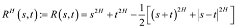
The covariance function ![]() is given by
is given by
![]() (6)
(6)
where ![]() is an even function. By (6) and Taylor expansion, we verify that
is an even function. By (6) and Taylor expansion, we verify that![]() , as
, as![]() , where
, where![]() . It follows that
. It follows that![]() . Also, by using (6) and the Taylor expansion again, we also have
. Also, by using (6) and the Taylor expansion again, we also have
![]() (7)
(7)
Using Bochner’s theorem, ![]() has the following stochastic integral representation
has the following stochastic integral representation
![]() (8)
(8)
where W is a complex Gaussian measure with control measure ![]() whose Fourier transform is
whose Fourier transform is![]() . The measure
. The measure ![]() is called the spectral measure of
is called the spectral measure of![]() .
.
Since![]() , the spectral measure
, the spectral measure ![]() of
of ![]() has a continuous density function
has a continuous density function ![]() which can be represented as the inverse Fourier transform of
which can be represented as the inverse Fourier transform of![]() :
:
![]() (9)
(9)
We would like to prove that f has the following asymptotic property
![]() (10)
(10)
where ![]() is an explicit constant depending only on H.
is an explicit constant depending only on H.
In the following we give a direct proof of (10) by using (9) and an Abelian argument similar to that in the proof of Theorem 1 of [16] . Without loss of generality, we assume that![]() . Applying integration-by-parts to (9), we get
. Applying integration-by-parts to (9), we get
![]() (11)
(11)
with
![]() (12)
(12)
We need to distinguish three cases:![]() ,
, ![]() and
and![]() . In the first case, it can be verified from (12) that
. In the first case, it can be verified from (12) that![]() , hence
, hence![]() , and
, and
![]() (13)
(13)
We will also make use of the properties of higher order derivatives of![]() . It is elementary to compute
. It is elementary to compute ![]() and verify that, when
and verify that, when![]() , we have
, we have
![]() (14)
(14)
and ![]() as
as ![]() which implies
which implies![]() .
.
The behavior of the derivatives of ![]() is simpler when
is simpler when![]() . (12) becomes
. (12) becomes
![]() (15)
(15)
and
![]() (16)
(16)
Hence, we have![]() ,
, ![]() , and both
, and both ![]() and
and ![]() are in
are in![]() .
.
When![]() , it can be shown that (14) still holds, and
, it can be shown that (14) still holds, and ![]() as
as![]() .
.
Now, we proceed to prove (10). First, we consider the case when![]() . By a change of variable, we can write
. By a change of variable, we can write
![]() (17)
(17)
Hence,
![]() (18)
(18)
Let ![]() be a fixed constant. It follows from (13) and the dominated convergence theorem that
be a fixed constant. It follows from (13) and the dominated convergence theorem that
![]() (19)
(19)
On the other hand, integration-by-parts yields
![]() (20)
(20)
By Riemann-Lebesgue lemma,
![]() (21)
(21)
Moreover, since ![]() by (13) and
by (13) and ![]() as
as![]() , we have
, we have ![]() as
as![]() . It follows that
. It follows that
![]() (22)
(22)
Then for all ![]() large enough, we derive
large enough, we derive
![]() (23)
(23)
Hence, we have
![]() (24)
(24)
Combining (18), (19), and (24), we have
![]() (25)
(25)
Then we see that, when![]() , (10) holds with
, (10) holds with![]() .
.
Secondly, we consider the case![]() . Since
. Since ![]() is continuous and
is continuous and![]() , (19) becomes
, (19) becomes
![]() (26)
(26)
Using (20) and integration-by-parts again we derive
![]() (27)
(27)
It follows from the (27), (16) and Riemann-Lebesgue lemma that
![]() (28)
(28)
We see from the above and (17) that
![]() (29)
(29)
This verifies that (10) holds when![]() .
.
Finally we consider the case![]() . Note that (19) and (24) are not useful anymore and we need to modify the above argument. By using integration-by-parts to (11) we obtain
. Note that (19) and (24) are not useful anymore and we need to modify the above argument. By using integration-by-parts to (11) we obtain
![]() (30)
(30)
Note that we have![]() . Hence
. Hence ![]() is integrable in the neighborhood of
is integrable in the neighborhood of![]() . Consequently, the proof for this case is very similar to the case of
. Consequently, the proof for this case is very similar to the case of![]() . From (30) and (14), we can verify that (10) holds as well and the constant
. From (30) and (14), we can verify that (10) holds as well and the constant ![]() is explicitly determined by H. Hence we have proved (10) in general.
is explicitly determined by H. Hence we have proved (10) in general.
It follows from (10) and Lemma 1 of [17] (see also [12] for more general results) that ![]() is strongly locally
is strongly locally ![]() -nondeterministic on any interval
-nondeterministic on any interval ![]() with
with ![]() in the following sense: There exist positive constants
in the following sense: There exist positive constants ![]() and
and ![]() such that for all
such that for all ![]() and all
and all![]() ,
,
![]() (31)
(31)
Now we prove the strong local nondeterminism of ![]() on I. To this end, note that
on I. To this end, note that ![]() for all
for all![]() . We choose
. We choose![]() . Then for all
. Then for all ![]() with
with ![]() we have
we have
![]() (32)
(32)
Hence, it follows from (31) and (32) that for all ![]() and
and![]() ,
,
![]() (33)
(33)
where![]() . This proves Theorem 1.
. This proves Theorem 1.
Funding
Supported by NSFC (No. 11201068) and “The Fundamental Research Funds for the Central Universities” in UIBE (No. 14YQ07).