1. Introduction
We explore here the implications of assuming a complex Riemannian geometry as a generalized theory of gravity. We find that the electromagnetic field naturally appears as the imaginary part of the metric tensor and that two other fields also emerge, denoted as S and W. This paper presents the concepts of complex Riemannian geometry and derives the Christoffel symbols, the E & M field equation and the two additional fields. While the overall geometry is based on complex numbers, each of the four fields is pure real. They are gravity gμν, E & M fμν and two new fields Sμνρ and Wμνρ. The next paper derives the Bianchi identities and the generalized Einstein tensor which can be used to provide field equations.
We note that there have been numerous attempts to embed electromagnetism into Riemannian geometry of which the most well known are Weyl’s gauge field [1] , Kaluza’s fifth dimension [2] and Eddington’s affine geometry [3] . Even exploration of making the metric tensor complex (as we propose here) was explored almost a hundred years ago by Mie [4] and Reichenbacher [5] . These two did not have general relativity available at that time, and their theories led nowhere.
This research began with a single goal: to explore a complex Riemannian geometry in the context of general relativity. It found that the E & M field equations appear automatically as well as two more fields which act as charge and energy sources. This paper lays the foundation for the complex geometry and the next paper presents the generalized Bianchi identities and Einstein tensor.
2. Hermitian Metric Tensor
Since general relativity has been a successful theory of gravity, any generalization should reduce to the standard theory in certain approximations. Hence in exploring complex Riemannian geometry, there is strong motivation to include an axiomatic structure which closely parallels the familiar Riemannian geometry. A reference text on General Relativity will be useful to some readers to fill in details of some steps, for the structure of that formulation applies in broad terms. An example of a suitable text would be Introduction to General Relativity by Adler, Bazin and Schiffer (ABS) [6] , but there are many available.
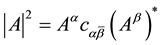
We begin with a complex Hermitian metric tensor  which defines an inner product between covariant complex vectors. The barred index is meant to indicate a complex-conjugate index, so that the inner product will be real as defined in Equation (2.1), where * indicates complex conjugation.
 (2.1)
(2.1)
This form of  can be written as a sum of its real and imaginary parts as shown in Equation (2.2a) with its Hermitian inverse
  also decomposed into real and imaginary parts as shown in Equation (2.2b). We note that since the two indices are typed for the complex metric tensors
  and
and , the indices can be in any order without confusion such as
  and
and ―a convention that will simplify some of the later equations. We will also use the same convention for
  and its raised form
 . Since the real part of
  and
and  are symmetric, typing is not required for those two (
 and
and ).
).
 (2.2a)
 (2.2b)
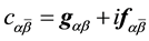
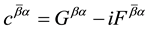
Here g is the usual symmetric metric tensor and f is an antisymmetric tensor. We will use bold font for those two basic fields, (gαβ and fαβ) as well as the two others (S and W), which naturally appear later. Thus it will be easy for the reader to identify the key fields. One may correctly surmise from this notation that f will be identified with electromagnetism. Since Gβα is not the inverse of gαβ due to the impact of the imaginary part fαβ, we will use the standard notation gβα for the inverse of gαβ. With this definition, we list some algebraic relationships in Equations (2.2c)-(2.2g). By expanding the equation ![]() into real and imaginary parts, we can derive (2.2c)-(2.2e). Multiply Equation (2.2c) by gγβ to get Equation (2.2f) and likewise multiply Equation (2.2d) by gγβ to get Equation (2.2g).
into real and imaginary parts, we can derive (2.2c)-(2.2e). Multiply Equation (2.2c) by gγβ to get Equation (2.2f) and likewise multiply Equation (2.2d) by gγβ to get Equation (2.2g).
Equation (2.2f) shows that ![]() equals gαβ except for terms second order and higher in
equals gαβ except for terms second order and higher in![]() . When we limit our consideration to second order terms,
. When we limit our consideration to second order terms, ![]() can be replaced by gαβ.
can be replaced by gαβ.
Using this result, Equation (2.2g) shows that ![]() equals
equals ![]() except for terms third order and higher in
except for terms third order and higher in![]() . Thus when we limit our consideration to second order terms,
. Thus when we limit our consideration to second order terms, ![]() can be replaced by the familiar raised form of the E & M tensor, fαβ.
can be replaced by the familiar raised form of the E & M tensor, fαβ.
![]() (2.2c)
(2.2c)
![]() (2.2d)
(2.2d)
![]() (2.2e)
(2.2e)
![]() (2.2f)
(2.2f)
![]() (2.2g)
(2.2g)
Raising and Lowering Indices: The metric tensor is customarily used for raising and lowering indices of vectors and tensors, and this property also applies to the Hermitian metric with one caveat―the conjugate quality of the index switches. Thus ![]() applied to Aα gives
applied to Aα gives ![]() and vice versa as summarized in Equations (2.3)-(2.4). One implication is that barred indices must be contracted with barred indices, and unbarred with unbarred. We identify
and vice versa as summarized in Equations (2.3)-(2.4). One implication is that barred indices must be contracted with barred indices, and unbarred with unbarred. We identify ![]() as the matrix inverse of
as the matrix inverse of![]() , one being used for raising indices and the other for lowering. This definition makes raising and lowering indices inverse operations as usual.
, one being used for raising indices and the other for lowering. This definition makes raising and lowering indices inverse operations as usual.
![]() (2.3a)
(2.3a)
![]() (2.3b)
(2.3b)
We also assume that one can convert between barred and unbarred indices by complex conjugation, i.e. you can create a new tensor with indices of flipped type by taking the complex conjugation of a previous tensor.
![]() (2.4a)
(2.4a)
![]() (2.4b)
(2.4b)
3. Covariant Derivative
We begin with scalar differentiation. In classical relativity, the partial derivative and the covariant derivative of a scalar field ϕ are the same numerically and are denoted respectively as ![]() and
and![]() , according to a familiar notation. We keep the same assumption here. Both types of scalar derivatives are numerically equal, as shown in Equation (3.1), but will differ on subsequent covariant derivatives according to their type.
, according to a familiar notation. We keep the same assumption here. Both types of scalar derivatives are numerically equal, as shown in Equation (3.1), but will differ on subsequent covariant derivatives according to their type.
![]() (3.1)
(3.1)
Vector Differentiation: Complex geometry can also introduce covariant differentiation with Christoffel symbols in the standard fashion, where there are now two different types of indices for the vector and two for the derivative resulting in four different types of Christoffel symbols shown in Equations (3.4a)-(3.4d).
![]() (3.2a)
(3.2a)
![]() (3.2b)
(3.2b)
![]() (3.2c)
(3.2c)
![]() (3.2d)
(3.2d)
We note that the Christoffel symbols for the lowered indices can be derived from Equations (3.3a)-(d) using ϕ = AνAν and Equation (3.1) for the covariant derivative of a scalar function―just as is frequently done in classical Riemannian geometry. The process is summarized in Equations (3.3a)-(3.3c). In Equation (3.3a) the scalar function AαBα is differentiated first as a scalar function as then as a tensor product. By expanding out the covariant derivatives in Equation (3.3b) and then reorganizing terms in Equation (3.3c), we get an equation for arbitrary tensor fields Aα and Bα. Since Aα is arbitrary, the other factor must be zero, and can be rewritten as Equation (3.4a). Similar logic leads to Equations (3.4b)-(3.4d).
![]() (3.3a)
(3.3a)
![]() (3.3b)
(3.3b)
![]() (3.3c)
(3.3c)
![]() (3.4a)
(3.4a)
![]() (3.4b)
(3.4b)
![]() (3.4c)
(3.4c)
![]() (3.4d)
(3.4d)
Note that with all derivatives of a vector, the vector index is always contracted with one of the first two indices of the Christoffel symbol, which two indices are always of the same type (barred or unbarred). The last index is always the derivative index.
We also require that covariant differentiation maintain conjugation symmetry. This last statement means that:
![]() (3.5a)
(3.5a)
and
![]() (3.5b)
(3.5b)
Equations (3.5a) and (3.5b) imply conjugation symmetry on the Christoffel symbols, namely:
![]() (3.6a)
(3.6a)
![]() (3.6b)
(3.6b)
We will frequently need to use the explicit difference between the barred and unbarred Christoffel symbols, and thus we give it its own symbol S as defined in Equation (3.7a) and (3.7b). Since the difference between two Christoffel symbols transforms as a tensor under coordinate transformations, we know that S must be a tensor. However, the third index―is slashed to indicate that it is neither barred nor unbarred since it is the difference between a barred and unbarred quantity. This distinction is only temporary to allow the derivation of the Christoffel symbols, and it will go away once the full solution is done.
![]() (3.7a)
(3.7a)
![]() (3.7b)
(3.7b)
We note one immediate corollary to this definition of S in (3.8a) or equivalently in Equation (3.8b).
![]() (3.8a)
(3.8a)
![]() (3.8b)
(3.8b)
Christoffel Symmetry Condition: Since we want this new geometry to reduce to classical Riemannian geometry when the metric tensor is pure real, we want to impose symmetry conditions on the Christoffel symbols which map to the classical symmetry in the last two indices. This is easily done in the cases where the last two indices are the same type which leads to symmetry conditions (3.9a) and (3.9b) which are complex conjugates of each other. Symmetry (3.9a) is the same one usually assumed for classical relativity.
![]() (3.9a)
(3.9a)
![]() (3.9b)
(3.9b)
Choosing the Symmetry Condition for Different Types of Indices: The open question is what symmetry condition to use when the last two indices are of different type. The two candidate symmetry conditions are (3.10a) and (3.10b). The first requires equality when transposing the last two indices, and the second requires complex conjugation. Initially neither one appears more compelling than the other, and both will reduce to the classical symmetry in the limit of real Christoffel symbols. We have explored both, and find that the second symmetry condition has no solution except a constant field for the imaginary part of the metric tensor. The first one, however, leads to the electromagnetic field and two other fields. The simple transpose symmetry also maps easily to all other forms of Christoffel symbols and enables Bianchi identities. It seems to be the obvious choice and is assumed here (Bianchi identities are derived in the next paper).
Transpose symmetry:
![]() (3.10a)
(3.10a)
Conjugate symmetry:
![]() (3.10b)
(3.10b)
Zero Derivatives for the Metric Tensor: The last requirement we want to make on the Christoffel symbols is that the covariant derivative of the metric tensor vanishes as usual. Since there are two types of covariant derivative, we get two equations―which are just complex conjugates of each other (with a transpose of indices).
![]() (3.11a)
(3.11a)
![]() (3.11b)
(3.11b)
The E & M Field Equation: Once we have the transpose symmetry for the Christoffel symbols and the zero derivative Equations (3.11a)-(3.11b), we can derive the desired E & M field equation by antisymmetrizing (3.11a) i.e. summing over all signed permutations of ρ, ν and γ (this is denoted {・・・} ρ, ν, γ). Since the Christoffel symbols are all symmetric in the lower indices, all the Christoffel terms vanish, leaving only one term in (3.12).
![]() (3.12)
(3.12)
Expanding that metric tensor in (3.12), we get further simplification in Equation (3.13) since the symmetric ![]() term drops out in the antisymmetrization. What is left is the standard E & M field equation which serves as a necessary condition for the Christoffel symbols to have a nonzero solution.
term drops out in the antisymmetrization. What is left is the standard E & M field equation which serves as a necessary condition for the Christoffel symbols to have a nonzero solution.
![]() (3.13a)
(3.13a)
We note that this field equation is well known to imply that the E & M field tensor ![]() can be expressed as the antisymmetric derivative of a vector potential Aρ as shown in Equation (3.13b) [6] . Either equation is equivalent to the other, and modern superconductivity theory, especially Josephson junctions, has shown that the vector potential is the real field [7] . Thus we could have this E & M field Equation (3.13a) satisfied simply by using Equation (3.13b) instead of
can be expressed as the antisymmetric derivative of a vector potential Aρ as shown in Equation (3.13b) [6] . Either equation is equivalent to the other, and modern superconductivity theory, especially Josephson junctions, has shown that the vector potential is the real field [7] . Thus we could have this E & M field Equation (3.13a) satisfied simply by using Equation (3.13b) instead of![]() . This is often done in modern E & M calculations.
. This is often done in modern E & M calculations.
![]() (3.13b)
(3.13b)
What about Current Density? Equation (3.13) is usually combined with a charge density equation, which is the source equation for the E & M fields. That equation, however, is a field equation rather than a structural equation―i.e. an equation that determines the charge sources in terms of the other fields. The next paper addresses the field equations while this paper sets up the structure of the geometry.
Solving for the Christoffel Symbols in Equations (3.11a) and (3.11b): In order to solve for the Christoffel symbols, we begin with a familiar approach by rewriting Equations (3.11a)-(3.11b) using lowered Christoffel symbols defined in Equations (3.14) as
![]() (3.14a)
(3.14a)
![]() (3.14b)
(3.14b)
The zero covariant derivative conditions in Equations (3.11a)-(3.11b) become extremely simple using the lowered Christoffel symbols as shown in Equations (3.15a)-(3.15b), where we drop the bar in the partial derivative of (3.15b) since it has no impact there.
![]() (3.15a)
(3.15a)
![]() (3.15b)
(3.15b)
Christoffel Solution with Symmetry (3.9a): With this fore structure, we now solve for the Christoffel symbols beginning with the symmetry from Equation (3.10a), copied below. One obvious corollary of Equation (3.10a) is that the lowered Christoffel symbols must be symmetric in the last two indices as shown in Equation (3.17a). (3.17b) is the complex conjugate of (3.17a). Then to help us solve for the Christoffel symbols, we use the tensor ![]() (defined earlier in Equation (3.7a)) in Equation (3.17c) and its complex conjugate in (3.17d). Lowered index versions of Equations (3.17c) and d are given in (3.17e) and (3.17f).
(defined earlier in Equation (3.7a)) in Equation (3.17c) and its complex conjugate in (3.17d). Lowered index versions of Equations (3.17c) and d are given in (3.17e) and (3.17f).
![]() (3.10a)
(3.10a)
![]() (3.17a)
(3.17a)
![]() (3.17b)
(3.17b)
![]() (3.17c)
(3.17c)
![]() (3.17d)
(3.17d)
![]() (3.17e)
(3.17e)
![]() (3.17f)
(3.17f)
We can get another symmetry condition for the S tensor by differencing Equations (3.10a) and (3.10b) (copied below) to get (3.18a) which becomes (3.18b) by rearranging terms and applying the definition of the S tensor. By using the complex conjugation relationship in (3.17f), we get the final equation we need in (3.18c).
![]() (3.10a)
(3.10a)
![]() (3.10b)
(3.10b)
![]() (3.18b)
(3.18b)
![]() (3.18b)
(3.18b)
![]() (3.18c)
(3.18c)
The two key equations used to discover the form of the S tensor are (3.17e) and (3.18c), which we repeat here in slightly more convenient form as Equations (3.19a) and (3.19b). This equations show that we have symmetry in the second two indices and conjugation symmetry in the first two indices.
![]() (3.19a)
(3.19a)
![]() (3.19b)
(3.19b)
First we can solve for the imaginary part then the real part of S. The imaginary part is symmetric in indices 2 and 3 (Equation (3.19a)) while antisymmetric in indices 1 and 2 (Equation (3.19b)). The only solution for the imaginary part is thus zero as shown in Equation (3.19c), where the imaginary part of S is shown to equal minus itself.
![]() . (3.19c)
. (3.19c)
From the same equations, the real part is symmetric in indices 2 and 3 as well as 1 and 2. The most general solution is an arbitrary, fully symmetric third rank real matrix. All permutations of the three indices must give the same real value for S. We denote this homogeneous solution as![]() . Since S has been shown to be pure real, from complex conjugation in Equation (3.17f),
. Since S has been shown to be pure real, from complex conjugation in Equation (3.17f),![]() .
.
![]() (3.20)
(3.20)
This result for S allows us to write the zero derivative condition on the metric tensor (Equation (3.10a)) in an equivalent form below which is much easier to solve. Simply subtract and add ![]() to Equation (3.10a) as shown in Equation (3.21a). Then use the definition of the S tensor to replace the first term with
to Equation (3.10a) as shown in Equation (3.21a). Then use the definition of the S tensor to replace the first term with ![]() as shown in (3.21b). Finally, replace the first Christoffel symbol with its conjugate form, and then move 2Sβαγ to the right side to give (3.21c).
as shown in (3.21b). Finally, replace the first Christoffel symbol with its conjugate form, and then move 2Sβαγ to the right side to give (3.21c).
![]() (3.21a)
(3.21a)
![]() (3.21b)
(3.21b)
![]() (3.21c)
(3.21c)
One can thus solve Equation (3.21c) also by considering first the real then the imaginary part. To solve for the real part we note that the real part of the left side of Equation (3.21c) is symmetric in α and β. The result for the real part ![]() is found in the same way as in standard Riemannian geometry (adding and subtracting cyclic permutations and using the index symmetry in Γ and g). The result is given in Equation (3.22), easily verified by substitution into the real part of Equation (3.21c).
is found in the same way as in standard Riemannian geometry (adding and subtracting cyclic permutations and using the index symmetry in Γ and g). The result is given in Equation (3.22), easily verified by substitution into the real part of Equation (3.21c).
![]() (3.22)
(3.22)
To solve for the imaginary part of ![]() we begin by rewriting the imaginary parts of Equations (3.21c) and (3.17a) to give:
we begin by rewriting the imaginary parts of Equations (3.21c) and (3.17a) to give:
![]() (3.23a)
(3.23a)
![]() (3.23b)
(3.23b)
The full solution for the imaginary part of the Christoffel symbol is given in Equation (3.24) and includes another arbitrary fully symmetric real matrix of third rank we call Wαβγ, as summarized in Equation (3.25). Note that the E & M field Equation (3.13a) is required to make this solution work.
![]() (3.24)
(3.24)
![]() (3.25)
(3.25)
This solution can be verified by substitution. The lack of any more degrees of freedom can be verified by looking for solutions of Equations (3.23) where f vanishes (i.e. the homogeneous equation). When f vanishes, those two Equations (3.23) mean that all such solutions are symmetric under interchanges of the first two and last two indices. By applying this rule twice, any solution must also be unchanged under exchange of the first and last indices. Thus any solution of the homogenous equation is a completely symmetric third rank matrix, which the added term of ![]() already includes. One concludes that Equation (3.24) and (3.25) together form the most general solution.
already includes. One concludes that Equation (3.24) and (3.25) together form the most general solution.
Christoffel Solution: Assembling all the pieces, the full solution to ![]() is given in (3.26).
is given in (3.26).
![]() (3.26)
(3.26)
The first term in Equation (3.26) is the classical lowered Christoffel symbol, a fact we shall use shortly to simplify the result. If it were subtracted from the left side (also a lowered Christoffel symbol), then we use the principle that the difference between two Christoffel symbols must transform as a tensor under coordinate transformations. Since S has already been proven to be a tensor, this means that the f and W terms together will transform as a tensor. Now W as defined in Equation (3.26) cannot be a tensor because the other term ![]() does not itself transform as a tensor. However, if we can add a fully symmetric pure imaginary
does not itself transform as a tensor. However, if we can add a fully symmetric pure imaginary
term to ![]() which can make it into a covariant tensor, then we can subtract the same term from W
which can make it into a covariant tensor, then we can subtract the same term from W
and define a new W which will be a tensor. Essentially we need to change the partial derivatives of f in Equation (3.26) to covariant derivatives.
Covariant Formulation: The choice to make is which covariant derivatives to use, which is the same as asking which Christoffel symbols to use? We require the Christoffel symbol selected to be real so that the redefined W stays pure real. The only option we have is to use the familiar Christoffel symbols of classical relativity― here written with bold green font ![]() to discriminate them clearly from the complex Christoffel symbols. Using the classical Christoffel symbols turns out to give a simple result, which provides a covariant and nonrecursive definition of the complex Christoffel symbols.
to discriminate them clearly from the complex Christoffel symbols. Using the classical Christoffel symbols turns out to give a simple result, which provides a covariant and nonrecursive definition of the complex Christoffel symbols.
To make the formalism easy to read, we use bold green font also to denote covariant derivative using the classical Riemannian Christoffel symbols, as in![]() .
.
The required term to create a covariant form is given in Equation (3.27). It is fully symmetric in (α, β, γ) plus purely imaginary and thus can be incorporated into the definition of W, which is an arbitrary fully symmetric additional field.
![]() (3.27)
(3.27)
We added and subtracted ΔTαβγ in (3.28a) and then rewrote the result in a more convenient form in Equation (3.28b) where we absorb the ΔT into the W field as we planned above and wrote the first term explicitly the lowered classical Christoffel symbol. The resulting W field is now bolded since it will be a real covariant field just like g, f and S. Equations (3.29a) and (3.29b) simplify the result even more by combining the first two terms using the complex metric tensor.
![]() (3.28a)
(3.28a)
![]() (3.28b)
(3.28b)
To complete the reformulation of this solution in Equation (3.28b) into an obviously covariant form, we need the algebraic result summarized in Equation (3.29), which simply uses the definition of the covariant derivatives above combined with the standard E & M field equation in Equation (3.13a).
![]() (3.29)
(3.29)
Substituting Equation (3.29) into Equation (3.28b), we get the result (3.30a).
![]() (3.30a)
(3.30a)
Since![]() , we rewrite Equation (3.30a) as Equation (3.30b).
, we rewrite Equation (3.30a) as Equation (3.30b).
![]() (3.30b)
(3.30b)
From this one equation we can use the definition of the S tensor (Equation (3.7a)) to find ![]() in Equation (3.31b). Complex conjugation then gives the next two Christoffel symbols in Equations (3.31c) and (3.31d).
in Equation (3.31b). Complex conjugation then gives the next two Christoffel symbols in Equations (3.31c) and (3.31d).
![]() (3.31a)
(3.31a)
![]() (3.31b)
(3.31b)
![]() (3.31c)
(3.31c)
![]() (3.31d)
(3.31d)
We can use these equations and the definition of S in Equation (3.7a) to compute S, and we find (not surprisingly) that all the S terms in Equations (3.31a)-(3.31d) are the proper S term for each Christoffel symbol.
Simplifying the Christoffel Equations with a Sign Convention for S and W Tensors: The Equations (3.31a)-(3.31d) all use one form of S and one form of W where only the second index is barred. If we define the S and W sign convention with barred indices, then a single formula will define all Christoffel symbols. In providing this sign convention, we must remember that the sign of the first two indices are always of opposite type, so there are only four combinations to consider―the type of the first and third indices.
We thus summarize the sign rule for the S tensor:
The S tensor changes sign if the type of the first two indices flip or the third index switches.
![]() (3.32)
(3.32)
This sign convention is consistent with the definition of S in Equation (3.17c) and the fully symmetric form of the index permutations of S for a fixed type from Equation (3.20).
We can also do a similar simplification with the W tensor.
The W tensor changes sign if the type of the first two indices switches (they are tied together). Index type makes no difference in the last index for W.
![]() (3.33)
(3.33)
Similarly, we note that ![]() is the imaginary part of a typed Hermitian matrix
is the imaginary part of a typed Hermitian matrix![]() , which means that
, which means that![]() . Using that sign symmetry we get the very simple result in Equation (3.34a) for the Christoffel symbol, where the type of index a determines the sign of the f terms. The raised formula is shown in (3.34b), where the type of index d (opposite to index c) determines the sign of the f term.
. Using that sign symmetry we get the very simple result in Equation (3.34a) for the Christoffel symbol, where the type of index a determines the sign of the f terms. The raised formula is shown in (3.34b), where the type of index d (opposite to index c) determines the sign of the f term.
![]() (3.34a)
(3.34a)
![]() (3.34b)
(3.34b)
4. Summary
This paper introduces the theory of complex Riemannian geometry and shows that the imaginary part of the metric tensor satisfies the field equation for E&M theory. In addition, two more real fields, denoted S and W also appear naturally in the process suggesting a pathway to a four-field geometry. The general formula for the Christoffel symbols is derived and the lowered Christoffel symbol separates out the four types of fields into distinct terms.
5. Discussion
This exploration has suggested a path where gravitational theory is generalized to naturally include four types of interaction. The next paper will carry the geometry further to include Bianchi identities and a generalization of the Einstein tensor equation―now with sources due to the other three fields. Whether this direction following nature is undetermined, it does provide a formalism and conceptual framework to explore this geometry further.