1. Introduction
The riddle of Time’s Arrow is an outstanding problem in modern physics. How does it come that we can remember yesterday but not tomorrow? Why do we all grow older but never grow younger? We all know that what is possible in one direction of time may be quite impossible in the other. The riddle of time consists in the observation that this asymmetry disappears when we turn to the microlevel: here, the all processes seem to be equally possible in both directions of time. So, if the fundamental laws of physics are time-symmetric, where does time asymmetry come from?
Ever since the time of Boltzmann [1] , it has been clear that this has something to do with entropy and the Second Law of Thermodynamics, although it is still not quite clear exactly what the relation is. In spite of a large number of different attempts to explain the asymmetry of time, there has been so far no agreement at all even about where to look for the solution: is it a question about the dynamical laws or about the boundary conditions of the universe? Is it a quantum mechanical problem or is it an essentially classical question about probabilities?
It is also not clear what it will mean to have an answer to the riddle. Of course, if it will be something simple, like an asymmetry in the dynamical laws which we have for some reason previously overlooked, then this will perhaps not be a problem. But if it is, as will be suggested in this paper, a probabilistic property of our universe, then the situation is different. In most cases, physical theories should try to describe as many details and factors as possible. In view of the enormous complexity of the universe, however, this may not be a possible strategy to start within the present case. Rather, we are forced by necessity to take the opposite path: to simplify as far as possible and discard everything which is not absolutely indispensable in order to reveal the underlying mechanism.
Another complication may be the concept of entropy itself. Under ordinary circumstances, entropy may be a fairly well understood concept. But it should always be remembered that it is developed in classical thermodynamics, and is best understood in stationary or quasi-stationary situations. This is very far from what we meet in cosmology, where some of our ordinary physical concepts get a new twist.
Still, another specific problem with Time’s Arrow seems to be that our very human perspective tends to make us formulate the questions in the wrong way, and that many of our conclusions may in fact already be unconsciously built into our assumptions (see Price [2] ). For this reason, it seems important to start the investigation by formulating some of these fundamental questions which underlie the discussions. In Sections 2 and 3, we, therefore, review three such assumptions. In Section 4, we study a very simple model for a semi-classical multiverse, and in Section 5 we apply Boltzmann’s ideas to relate the dynamics of it to the concept of entropy. A fundamental problem in this context is that we really do not know what we should mean by a state of the multiverse and how we should count them. In Section 6, we then turn this multiverse into a probability space by adding some assumptions about probability weights, and in Section 7 we discuss a non-technical argument why a monotonic growth of the entropy should be more likely than a symmetric behavior with low entropy at both ends. This is related to the old discussion originating from Gold’s famous paper [3] and continued by Hawking, Page, LaFlamme and others (see [4] [5] ), but from a rather different perspective.
In any case, these arguments are just the beginning of what should be done. Finally, in Section 8, we discuss how these ideas can be further developed.
Some of the ideas in this paper have been discussed earlier in a more preliminary and technical form in [6] , where some related ideas can also be found.
2. Our Underlying Assumptions
Examples of fundamental questions underlying the discussion are:
・ Is temporal causality a fundamental property of nature?
・ Is our universe unique? (instead of just one of many parallel ones?)
・ Is our world an infinite structure?
Depending on what answers, yes or no, we give to these questions, we get eight different perspectives on physics in general and on Time’s Arrow in particular. From our present state of knowledge, it is hard to argue that any one of these perspectives is obviously wrong or obviously the correct one. But it can still be very im- portant to be aware of which perspective we choose and why. The starting point for this paper is to assume that the answers to these questions are all no.
Temporal causality refers to the idea that events are somehow caused by previous events in the backward light-cone of the given event, and hence that the latter should be considered to be a consequence of these. From a human perspective, this may all be very natural. But from the point of view of fundamental physics, this is quite problematic. As has many times been pointed out by Price [2] , if we accept that the laws of physics are essentially time-symmetric, then there is no obvious reason why we could not equally well consider the given event as a consequence of events in the forward light-cone instead, since the equations of motion can in general equally well be solved backwards and forwards in time.
Temporal causality is very closely related to the question of Time’s Arrow. In fact, assuming temporal causality is more or less equivalent to taking a preferred direction of time for granted, which will obviously not do for an explanation of Time’s Arrow. There are several ways to try to get around this problem. First, we can of course deny the time-symmetry of the laws of physics. Or we can assume that the laws are symmetric, but that it is somehow a question about the boundary conditions of the universe. Both ways have been attempted by many authors, but so far without any obvious success (see e.g. [7] [8] ). In this paper, we instead make the assumption that both laws and boundary conditions are time-symmetric, but it will be argued that this can still lead to what we perceive as a directed Arrow of Time.
We will also assume that our universe is just one of many, and that this is the most natural interpretation of quantum mechanics. This is a question where the scientific community is clearly divided. But in most cases, our descriptions and predictions will be equivalent. However, one can note that in this context, accepting or not accepting the multiverse really will imply a difference: the explanation for Time’s Arrow in this paper does make natural sense in the multiverse, but it does not seem to do so if we insist on just a single universe.
As for the third question, the situation is still more complicated. One of the purposes of this paper is to argue that the different answers which we can choose to this question may generate very different pictures of reality in general and of Time’s Arrow in particular. And that this aspect is often forgotten in the discussion.
The use of infinities has a long history in science. They can easily be traced thousands of years back to Greek philosophers, like Zeno and Aristotle, and even further. Obviously, no single experiment has ever produced a truly infinite value, so what is it that makes the belief in infinities so strong?
At least part of the answer seems to be that in many cases infinities really do simplify our description of the world. There is an abundance of examples in any course in calculus or classical physics where studying a limit situation simplifies the problem tremendously.
Also, there is a kind of scale invariance argument for accepting infinities: to say that space-time is infinitely large and divisible into infinitely small parts in a sense amounts to saying that what we see on our intermediate level is exactly what we would see on any level of magnification which creates a, possibly illusory, feeling of complete understanding.
During the development of modern science, mathematicians and philosophers have had a lot to say about infinities, however without really having reached a state of consensus. Within physics the situation is somewhat different. Here one tends to accept infinities as long as we can make useful and consistent computations with them. Often, they are even regarded as powerful instruments in the toolbox, rather than as problems.
A rather trivial situation where assuming infiniteness tends to hide the real problem is the simple Martingale betting system and the so called St Petersburg paradox (see [9] ): suppose we play heads or tails and we win the stake if the coin comes up heads and lose it if the coin comes up tails. If we double our bet after every loss, the first win will recover all previous losses plus win an amount equal to the original stake. Thus, if we have access to an infinite amount of money, eventually heads will sooner or later come up and the Martingale betting strategy will always generate a gain in the long run if we go on in this way. But, of course, if the assumption about infinite wealth is removed then we will instead have to face the opposite fate of a certain ruin within a finite time. Clearly, assumptions about infiniteness in physics are usually much more subtle than in this example. Nevertheless, it can be that we are making similar mistakes in cosmology.
It may also be said that from a classical point of view, it was very natural to suppose the world to be infinite, simply because the perception of space-time was essentially based on the idea of real numbers. And once the infiniteness at one end of the scale is accepted, it is much easier to accept it at the other end too. With a quantum mechanical perspective, this is no longer true: within a finite volume, the quantum states will be discrete. Hence, the choice between finiteness and infiniteness essentially becomes the question whether the universe is closed or open.
3. Are the Underlying Assumptions in This Paper Compatible with Our Present Knowledge?
Concerning temporal causality, the present situation in science is that it is so deeply built into our way of thinking that it is very difficult to work without it. But on the fundamental level, temporal causality has been questioned by many. Some people even go as far as questioning the flow of time itself. Often, the starting point is the Wheeler-deWitt equation (see e.g. [10] - [12] ). However, the approach in this paper is in fact rather independent of all such attempts.
When it comes to the multiverse interpretation, originating from the work of Everett [13] , some people would say that simple physical experiments, where particles seem to interfere with themselves, should be considered as genuine proofs of the existence of parallel worlds. But of course, other interpretations are possible. Let us not enter this discussion here. Critics of the multiverse interpretation often focus on the tendency in recent times to expand this idea too far: there is an obvious risk that we will end up finding ourselves in a wonderland where everything is possible and nothing is certain. The point of view in this paper however, can rather be said to be the opposite one: an extremely simplified model where it should be possible to do computations and in the end prove rigorous results.
As for the third question about infinities, a possible interpretation of the situation is as follows: since the birth of modern cosmology about a hundred years ago, a number of different cosmological models have been proposed. For a long time, the closed Friedmann model (see [14] [15] ) was the most wide-spread model, but towards the end of the 20th century, open models became increasingly popular. When it was discovered in 1998 that the expansion of the universe is actually accelerating (see [16] [17] ), this was by many people interpreted as a very strong argument in favor of open models.
Although there are still critical voices, it is probably fair to say that the acceleration of the expansion is rather firmly established. But does this imply that the universe is open? This may in fact be another instance where our use of infinities mislead us. The conclusion is reached by extrapolating Einstein’s field equations with a cos- mological constant. But it can also be said that the very existence of the accelerating expansion itself seems to indicate that there might be something wrong with the field equations on a cosmological scale, so it might be rather dangerous to extrapolate them. In fact, an alternative explanation of the observed phenomena may be that it is the finiteness of the universe itself which causes that we now perceive as an accelerating expansion. For a more thorough discussion of these matters, see [18] .
So far the conclusion must be that, for the time being, we must leave all these three questions open. The best thing we can do is to analyze different models, and in the end hope that our understanding and comparison with measurements will single out one preferred theory.
4. The Finite Multiverse
One of the main points of this paper is that if we answer no to all the three questions in Section 2, a rather natural perspective on cosmology emerges. On the other hand, this perspective is not so easy to fit together with a yes to any of the questions.
To start with, a finite universe will be bounded, both in space and time. In fact, simplifying somewhat, we may assume that there are only a finite number of moments of time between the Big Bang and the (inevitable) Big Crunch. To make things as simple as possible, let us choose a time-axis between  (Big Bang) and
  (Big Crunch), such that these discrete moments of time correspond to the integers. And for each such moment of time, there will be only a finite number of possible states of the multiverse.
What these states are like and in what sense they are related to quantum mechanical states is a non-trivial question. The problem is that different states of the multiverse cannot be treated as quantum mechanical states in the usual sense for the following simple reason: time-development is unitary and therefore maps quantum mechanical states at one moment of time onto quantum mechanical states at another moment of time in an isomorphic way. Thus, a state now will always correspond to a unique state in the future. But the most characteristic property of the multiverse is that any state now can give rise to many different states in the future (in the following, this will be referred to this as the branching property of the multiverse). In the model of this paper, this property is lost if we consider ordinary quantum states.
It is perfectly possible to interpret states in a classical way, e.g. by splitting phase space into lots of small cells and consider a state to be determined by specifying which particles belong to which cells. Nevertheless, the world is after all quantum mechanical, so something is obviously lost here too. But if the states of the multiverse are neither classical nor quantum states, what are they then? In fact, it may very well be that there is no reasonable such concept. Perhaps the best compromise for the time being is to think of them as distinguishable configurations. Still, it may be illuminating to study a semi-classical approximation of the multiverse where states do make sense. This is very much in the tradition of physics where discrete approximation to continuous systems or continuous approximations to discrete systems are frequently used. Certainly, it is by no means evident that this extremely simplified way of thinking is good enough to reflect the true character of the world. Nevertheless, in this paper it will be consider as an adequate model for discussing Time’s Arrow.
As we pass from one moment of time to the next (or previous), the laws of physics will give different pro- babilities for a transition from one state to another. In general this is, on the scale of the whole multiverse, an enormously complicated process. But if we, following the philosophy in Section 1, simplify as much as we can,
then we may just classify each transition as possible or impossible.
In this way, we obtain something which is actually a enormous but finite graph: a node is simply a possible state at some moment of time and an edge connects states at adjacent moments of time such that the transition between them is possible. Note that we will always suppose that if a transition is possible in one direction of time, then it is also possible in the other, which corresponds to assuming that the dynamical laws are time- symmetric.
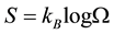
Definition 1 A universe U is a path, or a chain of states (one state Ut for each moment of time t), with the property that the transition between adjacent states is always possible.
Definition 2 The multiverse M is the set of all possible universes U in the sense of Definition 1 (see Figure 1).
5. Boltzmann in the Multiverse
To be able to say something about Time’s Arrow in the multiverse of the previous section, we also need to discuss entropy. My position in this paper is to try not to take more than necessary about entropy for granted. As a starting point, let us return to two well-known and fundamental ideas, both due to Boltzmann.
The first idea, as well as the foundation of the modern theory of entropy of a macro-state , is contained in Boltzmann’s famous formula [1] :
 , (5.1)
or alternatively
 . (5.2)
Here,  denotes the number of micro-states compatible with
 , and
, and  is Boltzmann’s constant.
Although this formula is usually derived under circumstances which are very far from what we meet in cosmology, it still represents a very fundamental truth. In the following it will always be assumed that in whatever way we measure the entropy S, the number of states corresponding to that entropy is an exponentially growing function of S as in (5.2).
The other fundamental idea of Boltzmann is that the second law of thermodynamics is a manifestation of the fact that the universe, as time develops, passes from less probable states to more probable ones. This idea is by no means less important than the first one. But as it stands, it is unfortunately rather useless for explaining Time’s Arrow, since it already has supposed direction of time built into it. Therefore, we need to reformulate Boltzmann’s second idea in a time symmetric form. To do this, the following points must be taken into account:
・ The dynamics must be time-symmetric.
・ The branching property of the multiverse must be included.
・ The relation to the entropy must be clear.
![]()
Figure 1. A schematic picture of a universe as one particular path from the Big Bang to the Big Crunch in the huge graph of all possible states.
The following formulation seems to include the essence of Boltzmann’s idea in a time-symmetric way:
Statistical Assumption Given any state of a universe, at any moment of time between the Big Bang and the Big Crunch, which is not very close to the end points and where the entropy is not close to being maximal, the number  of accessible states with higher entropy at the next/previous moment of time is very large, and the number of accessible states with lower entropy at the next/previous moment of time is very small (or rather, the probability
  for finding any such accessible state is very small). In the following,
  will be considered to be essentially independent of time and of the particular state.
Also it will always be assumed in the following that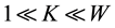 .
.
Near the end points, the dynamics may be quite different from the rest of the time (see the next section). At the end points  and
and , it will be assumed that there is only one state with zero volume and entropy.
If the entropy is maximal or close to, among all states at some moment of time , this assumption obviously has to be modified somewhat. But let us explicitly agree to not consider the life-span of the multiverse to be long enough for the entropy to become anything near to maximal, except possibly close to the end-points. In fact, according to [19] [20] , the entropy of our present universe is very far from maximal and may continue to be so for a very, very long time still.
Remark 1 Once ![]() and
and ![]() are determined, the
are determined, the ![]() in the Statistical Assumption above is also determined. To see this, consider for a given moment of time
in the Statistical Assumption above is also determined. To see this, consider for a given moment of time ![]() (or
(or![]() ), all states with entropy
), all states with entropy![]() . According to (5.2), there are
. According to (5.2), there are ![]() such states. For each of these states there are
such states. For each of these states there are ![]() accessible states with entropy
accessible states with entropy ![]() at time
at time![]() . Assuming statistical independence, we see that there are
. Assuming statistical independence, we see that there are ![]() accessible state with entropy
accessible state with entropy ![]() at time
at time![]() . Since there are in total
. Since there are in total ![]() such states, we conclude that only the ratio
such states, we conclude that only the ratio
![]() (5.3)
(5.3)
of these states can be accessible from states with lower entropy.
6. The Multiverse as a Probability Space
We can now make the multiverse into a finite probability space, using the Statistical Assumption of the previous section.
Thus, let ![]() be the time-interval from the Big Bang to the Big Crunch. It will be convenient in the following to split the life-span of the multiverse into three different phases: we choose symmetric moments of time
be the time-interval from the Big Bang to the Big Crunch. It will be convenient in the following to split the life-span of the multiverse into three different phases: we choose symmetric moments of time ![]() and
and ![]() close to the end-points of the interval
close to the end-points of the interval ![]() so that we can write
so that we can write
![]() . (6.1)
. (6.1)
Coarsely speaking, this may be thought of as a kind of idealized division into the extreme initial phase, the normal phase and the extreme final phase of the multiverse. It is difficult to have a definite opinion about how long the extreme phases should be, but it sounds reasonable to assume that the passage into the normal phase would occur somewhere close to the inflation.
We can now to each universe assign an (un-normalized) probability weight as follows:
![]() . (6.2)
. (6.2)
Here ![]() and
and ![]() represent the weights for the development from
represent the weights for the development from ![]() to
to ![]() and from
and from ![]() to
to ![]() re- spectively, whereas
re- spectively, whereas ![]() refers to the normal phase in between.
refers to the normal phase in between.
During the normal phase, according to the idea in Section 4, each transition is just classified as either possible or impossible, i.e. has weight 1 or 0. It follows that ![]() will be 1 for all universes. Let us also assume that we measure the entropy on an appropriate scale where it is reasonable, again as an extreme simplification, to assume that it can (during this phase) only change by
will be 1 for all universes. Let us also assume that we measure the entropy on an appropriate scale where it is reasonable, again as an extreme simplification, to assume that it can (during this phase) only change by ![]() per each unit interval of time.
per each unit interval of time.
During the extreme phases, the situation is very different. The volume will be very small and quantum effects dominate. Here, in a sense, everything can happen, although of course not with the same probability. On the other hand, the duration of the extreme phases is very short, so we will assume that the most probable scenario is that very little happens at all. To make this somewhat more formal, let us assume that a universe, starting from the unique state at time ![]() with zero entropy, can develop into any state at time
with zero entropy, can develop into any state at time![]() . But the probability for such a development will be given by an exponential distribution
. But the probability for such a development will be given by an exponential distribution
![]() , (6.3)
, (6.3)
where ![]() is a large constant. In other words, the probability for the universe to enter the normal phase in a disordered state decreases very rapidly with the entropy. The symmetric situation applies to the interval
is a large constant. In other words, the probability for the universe to enter the normal phase in a disordered state decreases very rapidly with the entropy. The symmetric situation applies to the interval![]() .
.
We now have made the multiverse into a probability space. Note however, that there are still several unspecified parameters, in particular ![]() and
and![]() .
.
7. Monotonic Universes Versus Universes with Low Entropy at the Ends
In this section, we finally turn to the question why the probability space in Section 6 should give rise to time asymmetry: the idea is that although the model itself is time symmetric, individual universes with a directed time could simply be much more probable than other relevant types. In other words, there could be an enormous number of different universes which share the same Big Bang and Big Crunch, and it could also be that in almost 50% of them the Arrow of Time points in the same direction as in our universe, and in almost 50% of them it points in the other direction. And the fact that we perceive an asymmetry of time could just reflect the fact that we can only observe the very small part of the multiverse to which we are confined.
To keep the discussion in this section as simple and non-technical as possible, let us just concentrate on comparing the total probability weight for universes with a monotonic behavior of the entropy (starting from approximately zero entropy at one end of the normal phase), with universes with low entropy at both ends of the normal phase. We let Pm be the total probability weight for a monotonic behavior and Ps be the corresponding probability weight for the-low-entropy-at-the-ends type of behavior. The task is to compute these two probability weights and then compare their sizes.
To start with![]() , the argument goes as follows: according to the statistical way of counting in Section 5 and the assumption that the entropy can only change by
, the argument goes as follows: according to the statistical way of counting in Section 5 and the assumption that the entropy can only change by![]() , a state with entropy 0 at time
, a state with entropy 0 at time ![]() can lead to K different states with entropy 1 one unit of time later. Each such state can again lead to K states with entropy 2 after two units of time, which gives a total of
can lead to K different states with entropy 1 one unit of time later. Each such state can again lead to K states with entropy 2 after two units of time, which gives a total of ![]() developments so far. Continuing in this way, we see that there are
developments so far. Continuing in this way, we see that there are ![]() developments with monotonically increasing entropy leading from the state with zero entropy at
developments with monotonically increasing entropy leading from the state with zero entropy at ![]() to states with entropy
to states with entropy ![]() at time
at time![]() . Each of these will according to (6.3) have a very small probability weight
. Each of these will according to (6.3) have a very small probability weight ![]() during the last extreme phase. It can be noted that this method of counting gives the same weight if we start from the
during the last extreme phase. It can be noted that this method of counting gives the same weight if we start from the ![]() states with entropy
states with entropy ![]() at time
at time ![]() and use the
and use the ![]() of Remark 1 to count backwards instead. Clearly, there are also equally many developments with decreasing entropy during the normal phase, so we arrive at
of Remark 1 to count backwards instead. Clearly, there are also equally many developments with decreasing entropy during the normal phase, so we arrive at
![]() (7.1)
(7.1)
Next we estimate![]() . According to our model, each universe with low entropy at both ends will be cha- racterized by transitions which increases the entropy by 1 at
. According to our model, each universe with low entropy at both ends will be cha- racterized by transitions which increases the entropy by 1 at ![]() moments of time and decreases it by
moments of time and decreases it by ![]() at equally many moments of time. As above, each transition of the first type will contribute to the number of universes by a factor
at equally many moments of time. As above, each transition of the first type will contribute to the number of universes by a factor![]() , and each transition of the second type will contribute (according to Remark 1) with a factor
, and each transition of the second type will contribute (according to Remark 1) with a factor![]() . Hence we get the number
. Hence we get the number
![]() (7.2)
(7.2)
of developments (in our case, this will give a very small number, thus the chance for finding any such universe is very small). The number of different choices of intervals where the entropy increases and decreases is obviously less than
![]() , (7.3)
, (7.3)
which together with (7.2) gives
![]() . (7.4)
. (7.4)
Again we note that we get the same result if we count in both directions of time. Hence,
![]() . (7.5)
. (7.5)
Summing up the discussion, we arrive at
Claim 1 If ![]() and
and![]() , then
, then![]() .
.
In other words, the chance for a behavior with low entropy at both ends in our probability space is very small compared to the chance for a monotonic behavior (Figure 2).
8. Discussion
The claim in Section 7 is deduced under extremely simplified premises and is obviously only the very begin- ning of what we should do if we want to pursue this path towards a deeper understanding of the Arrow of Time. In fact, recently there have been some progress in understanding and simulating Time’s Arrow in classical N- body systems with N of intermediate size, e.g. ![]() (see [21] ). This kind of system is certainly large enough to investigate time-asymmetry, although perhaps still not quite large enough to analyze entropy.
(see [21] ). This kind of system is certainly large enough to investigate time-asymmetry, although perhaps still not quite large enough to analyze entropy.
A natural question in connection with the model in this paper is: how about high entropy at both ends? It can of course be argued that this may not be directly relevant for the question of Time’s Arrow. After all, it seems to be a well established observational fact that we live in a universe with low entropy at least at one end, so the question is really about how such universes behave. Universes with high entropy at both ends are probably quite un-inhabitable, so maybe we should not bother about them?
Nevertheless, if we take the multiverse perspective seriously, it should be interesting to understand whether monotonic universes are the most common among all possible universes or not. To construct models where this is indeed the case may be more difficult than to deal with the simple-minded approach in this paper, at least if we want to make realistic assumptions. The Statistical Assumption in Section 5 must perhaps be replaced by something more complicated. In particular, it should be noted that the assumption in this paper endows the multiverse with a kind of Markov property: whatever happens before a certain moment of time ![]() is not im- portant for predicting the entropy at time
is not im- portant for predicting the entropy at time ![]() as long as we know the entropy of the present state. This is clearly
as long as we know the entropy of the present state. This is clearly
![]()
Figure 2. The two plots of entropy for probable universes represent the two kinds of scenarios included in Pm in (7.1). The plot of the unprobable universe represents one (of many) possible scenarios which are included in Ps in (7.4). The computation in (7.5) shows that in spite of the large number of different types of scenarios of type Ps, their total probability is very small under the assumption in Claim 1.
very unrealistic: many processes, e.g. light emanating from a source, can so to speak keep a memory of their origin for billions of years.
In addition to this, things like the inflation in the early universe may play an important role. Even more im- portant is probably the question about what states are and how we count them. This is also closely related to the question whether the expansion of the universe contributes to the growth of entropy or not. On the one hand, it can be said that this is just a question about definitions: entropy is just what we define it to be. But the real question is of course how to define entropy in a way which is compatible with the second law. And the answer to this question may very well depend on which part of the history of our universe we consider: the inflationary phase, the early universe or the full-grown universe where galaxies have essentially already formed.