1. Introduction
A Josephson junction (JJ) is a device consisting of two weakly coupled superconductors [1] . The dynamics of the superconducting phase difference ϕ across the junction is described by the Josephson equations [2] :
 (1a)
(1a)
 (1b)
(1b)
where I is the current flowing through the junction (IJ being the maximum value that can flow in the zero-voltage state), ħ = h/2π, h being Planck’s constant, and V is the voltage across the two superconductors. The above equations are named after b. d. Josephson, who received the Nobel Prize in 1973 for having predicted, through Equations (1a) and (1b), the so called d. c. and a. c. Josephson effects [1] . In the d. c. Josephson effect a non-dissipative current can be seen to flow at zero voltage, as it can be shown by setting V = 0 in (1b), so that ϕ = constant. In this way, IJ represents the maximum value of I flowing in the junction in the zero-voltage state. In the a. c. Josephson effect, the voltage across the JJ is kept at a fixed non-zero value V0. Integrating both sides of Equation (1b) we obtain , where ϕ0 is the constant of integration. Therefore the current I is seen to oscillate at a frequency
 . Equations (1a) and (1b) are derived from the special properties of superconductors, which we may recall here briefly. In 1911 Kamerlingh Onnes from Leiden first noticed that the resistivity of mercury (Hg) vanished completely below 4.2 K. Some other metals and compounds were observed to make the same transition from a “normal” state to a “superconducting” state below a critical temperature Tc which depended on the particular substance considered [3] . Years later, Meissner and Ochsenfeld [4] noticed that superconductors are perfect diamagnets; i.e., the magnetic induction is exactly zero in a superconducting region, so that M = −H and the magnetic susceptibility is μ = −1. The Bardeen, Copper and Schrieffer (BCS) theory of superconductivity [5] , published in 1957, finally established that condensation of electron pairs (Cooper pairs) in a coherent macroscopic state would explain most of the experimental properties of superconductors. A Cooper pair consists of two electrons with opposite spin and opposite momenta coupled via an effective electron-electron interaction mediated by lattice vibrations. The zero-spin Cooper pairs, possessing a boson nature, can all condensate in a macroscopic state whose wave-function is characterized by a complex number whose phase plays an important role in determining the superconducting properties, as we shall see, referring to Josephson junctions, in the following sections. After the BCS theory had been published, Josephson derived Equations (1a) and (1b) by means of a purely quantum mechanical analysis in 1963. Alternative derivations of the above equations have been also proposed by Feynman [6] and by Ohta [7] . In the Feynman model a JJ is described as a weakly coupled two-level quantum system. Ohta noticed that Feynman model did not include an additional term due to energy contribution of the external classical circuit biasing the Josephson junction. The latter author therefore introduced a semi-classical model based on a rigorous quantum derivation.
When Josephson junctions are in the presence of an external magnetic field, interesting phenomena, recalling diffraction and interference in optics [8] , are observed. In fact, in the same way a single slit lighted by a plane electromagnetic wave generates a Fraunhofer pattern on a distant screen, a single JJ in the presence of an externally applied magnetic field H shows a Fraunhofer-like pattern in the IJ vs. H curves [1] . On the other hand, the maximum current Ic which can be injected in a parallel connection of two JJs (a two-junction quantum interferometer) shows a magnetic field dependence qualitatively similar to the interference pattern seen in the Young’s two-slit experiment [8] . Furthermore, in a multi-junction quantum interferometer (a parallel connection of N JJs, with N > 2) the Ic vs. H curves are similar to those observed in the optical interference with N slits.
In the present work we shall therefore take a close look at these surprising parallelisms. In optics, of course, light itself provides the necessary oscillatory behavior, giving rise to interference phenomena. On the other hand, in superconducting systems the wavelike source is given by the macroscopic wave function describing the quantum state of each superconducting element in the JJ. On the basis of this analogy, in the following section we briefly review fluxoid quantization in a superconducting ring containing a Josepshon junction. In the third section the behavior of a single JJ in the presence of a magnetic field and the Fraunhofer-like pattern in the IJ vs. H curves are studied. In the fourth section two-junction quantum interferometers are seen to give Ic vs. H curves similar to the interference pattern seen in the Young’s two-slit experiment. In the fifth section quantum interference in a multi-junction quantum interferometer is considered in various examples. Conclusions are drawn in the last section.
2. Flux and Fluxoid Quantization
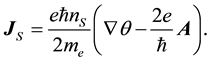
In discussing magnetic properties of Josephson junction devices, it is convenient to give a first brief look at flux and fluxoid quantization in multiply connected superconducting systems, by defining the current density JS of super-electrons flowing in a superconductor S. As in any other quantum system described by a wave function Ψ, the particle current density J in a superconducting system can be derived by considering Schroedinger equation for a free particle of mass m and the continuity equation, respectively reported below:
 (2a)
(2a)
 (2b)
(2b)
By expanding the time derivative in Equation (2b) and by considering Equation (2a), the expression of the supercurrent JS can be found to be
 (3)
(3)
where the vector potential A has been introduced by means of the minimal substitution  so that
 . It is now possible to consider the superconducting wave-function Ψ in a superconductor S expressed in terms of the number density of super-electrons ns and of the superconducting phase θ [9] :
 (4)
(4)
In this way, the supercurrent JS becomes:
 (5)
(5)
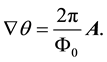
Considering now a multiply connected superconductor (a superconducting ring at the absolute temperature T below the critical temperature Tc) in the presence of a magnetic field H, along a path C well inside the superconductor we can consider JS = 0, so that:
 (6)
(6)
where  is the elementary flux quantum. By integrating both sides of Equation (6) over the path C, we get quantization of the flux Φ linked to the superconductor S:
 (7)
(7)
The quantized values of the trapped flux in a field cooling experiment (i.e., in a situation in which the superconductor temperature T is lowered from T > Tc to T < Tc in the presence of a magnetic field H) was given in terms of the applied field intensity H by Goodman and Deaver in 1970 [10] . The experimental results reported in ref. [10] can be summarized by the following simple non-linear expression: n = Ω(nex). The function Ω is such that, when applied to a real number x, gives the closest integer to x. This function can be easily interpreted by
considering the minima of the normalized magnetic energy , where
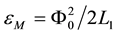 , L1 being
the inductance coefficient pertaining to the superconducting ring, ![]() , and
, and![]() , where μ0 is the magnetic permeability of vacuum and Sh is the area of the inner hole of the superconducting structure in which a magnetic field h is present. In fact, by fixing the value of the applied field (which, for a fixed area Sh, determines the value flux number nex), the system arranges itself in the quantized flux state with n trapped fluxons inside the hole that minimizes the magnetic energy εM.
, where μ0 is the magnetic permeability of vacuum and Sh is the area of the inner hole of the superconducting structure in which a magnetic field h is present. In fact, by fixing the value of the applied field (which, for a fixed area Sh, determines the value flux number nex), the system arranges itself in the quantized flux state with n trapped fluxons inside the hole that minimizes the magnetic energy εM.
Let us now consider a superconducting ring interrupted by a Josephson junction, as shown in Figure 1. We can think the JJ as a cut, consisting of a very thin insulating layer, between the two arms of the same superconducting ring. In this case, the line integral of the vector potential A over the path C well inside the superconductor needs to be calculated into two parts: the first inside the superconducting region S, where Equation (6) holds, the second across the thin insulating barrier B. Therefore, we have:
![]() . (8)
. (8)
By following the path C as prescribed by the right-hand screw rule, the first integral can be calculated in terms of the superconducting phase difference θ2 − θ1 across the JJ and the second can be opportunely labeled as in Figure 2, so that, by defining the gauge-invariant phase difference ϕ as follows
![]() (9)
(9)
![]()
Figure 1. A superconducting ring interrupted by a Josephson junction in the presence of a magnetic field. Well inside the superconductor S, along any of the paths shown, the supercurrent JS is zero. The middle path is labelled with the letter C. This path crosses the insulating barrier B (the cut within the ring) dividing S into two arms. We label the sides of the barrier as follows: side 1, where the currents enters the barrier B; side 2, from where the current leaves the barrier B.
![]()
Figure 2. A Josephson junction with a thin insulating barrier of length L, width w, and thickness t in the presence of a magnetic field H. Well inside the superconductors S1 and S2, along the path A1A2B2B1 the supercurrent JS is zero. The magnetic flux linked to the path shown is thus μHdΔx, d being the effective thickness of the barrier.
we can rewrite Equation (8) as follows:
![]() (10)
(10)
Equation (10) is similar to the flux quantization relation (7). However, one can immediately notice that the magnetic flux linked to path C is not quantized when the ring is interrupted by a JJ. Nevertheless, we can notice that the quantity![]() , which can be denoted as “fluxoid”, is still quantized.
, which can be denoted as “fluxoid”, is still quantized.
From Equation (10) we can also argue that magnetic flux Φ linked to a superconducting ring and the gauge- invariant superconducting phase difference ϕ across a Josephson junction interrupting the same ring are two intimately related quantities.
3. Josephson Junctions in the Presence of a Magnetic Field
We have seen that the gauge-invariant superconducting phase difference ϕ across a Josephson junction interrupting a superconducting ring is related to the magnetic flux trapped inside the same ring. When considering an isolated extended Josephson junction in the presence of a magnetic field, we may notice that a similar relation exists between ϕ and the flux linked to the barrier. This property leads us to the first type of quantum interference phenomenon: the Fraunhofer-like pattern in the maximum Josephson current I0 vs. H curves.
By referring to Figure 2, we assume that the field H is uniform along the length L of the JJ. We thus notice that the magnetic flux linked to the oriented rectangular path A1A2B2B1 is ![]() where, considering the penetration lengths l1 and l2 inside S1 and S2,
where, considering the penetration lengths l1 and l2 inside S1 and S2, ![]() is the effective barrier thickness. In this way, by calculating the line integral of the vector potential, one sees that
is the effective barrier thickness. In this way, by calculating the line integral of the vector potential, one sees that
![]() (11)
(11)
In the limit of![]() , we may write Equation (11) as follows:
, we may write Equation (11) as follows:
![]() (12)
(12)
where ![]() is the magnetic flux linked to the whole barrier. Being the term on the left-hand side
is the magnetic flux linked to the whole barrier. Being the term on the left-hand side ![]() a constant, the gauge-invariant superconducting phase difference ϕ is seen to vary linearly in the y-coordinate as follows:
a constant, the gauge-invariant superconducting phase difference ϕ is seen to vary linearly in the y-coordinate as follows:![]() , where ϕ0 is a constant to be determined. By assuming a uni- form current density J flowing in the JJ as shown in Figure 2, we may take the current-phase relation (1a) to be valid in an infinitesimal y-interval of length dy, so that we may write:
, where ϕ0 is a constant to be determined. By assuming a uni- form current density J flowing in the JJ as shown in Figure 2, we may take the current-phase relation (1a) to be valid in an infinitesimal y-interval of length dy, so that we may write:![]() . Therefore, by integrating the current over the junction barrier, one can find:
. Therefore, by integrating the current over the junction barrier, one can find:
![]() (13)
(13)
where![]() . The maximum Josephson current IJ flowing in the device can be found by maximizing the expression for I in Equation (13) with respect to ϕ0.
. The maximum Josephson current IJ flowing in the device can be found by maximizing the expression for I in Equation (13) with respect to ϕ0.
One thus finds:
![]() (14)
(14)
A graph of the above Fraunhofer-like function IJ/I0 is reported in Figure 3 (full line) along with the normalized Fraunhofer pattern ![]() (dashed line) for comparison. The similarity of these curves is evident, especially because the minima are located at the same positions, i.e. at nonzero integer values of the variables x and ΦJ/Φ0, as shown in the reported figure.
(dashed line) for comparison. The similarity of these curves is evident, especially because the minima are located at the same positions, i.e. at nonzero integer values of the variables x and ΦJ/Φ0, as shown in the reported figure.
![]()
Figure 3. Maximum Josephson current IJ normalized to I0 as a function of the normalize applied flux ΦJ/Φ0 (full line curve). For comparison, the Fraunhofer pattern (dashed curve) is shown.
4. Two-Junction Quantum Interferometers
In the present section we describe the similarity between the Ic vs. H curves for a two-junction quantum interferometer in the presence of a magnetic field H and the interference pattern seen in the Young’s two-slit experiment. Let us then consider the two-junction quantum interferometer schematically represented in Figure 4. This system consists of a current biased superconducting loop interrupted by two Josephson junctions, denoted as JJ1 and JJ2. The bias current IB is seen to split in two branch currents, I1 and I2. A magnetic field H is applied perpendicularly to the plane of the quantum interferometer. We may start our analysis by writing the fluxoid quantization condition for the system, so that:
![]() (15)
(15)
where ϕ1 and ϕ2 are the gauge-invariant superconducting phase differences across JJ1 and JJ2, respectively. The sign for the superconducting phase difference across JJ2 is negative, given that the oriented path around the superconducting loop crossing this junction opposes the assumed positive direction of the current I2.
We may also write the electrodynamic equation defining the flux Φ inside the loop as the sum of the induced flux and the applied flux![]() , S0 being the area of the loop. We may therefore set:
, S0 being the area of the loop. We may therefore set:
![]() (16)
(16)
where L is the self-inductance coefficient pertaining to a single branch. Notice that the magnetic flux induced by I1 and I2 are of opposite signs. Having defined these constraints, we may write down the dynamical equation for each Josephson junction in the loop. By adopting the Resistively Shunted Junction (RSJ) model [1] we may write:
![]() (17)
(17)
where the two junctions are assumed to be equal, so that they possess the same resistive parameter R and the same maximum Josephson current IJ, and where k = 1, 2. Notice that the terms in Equation (17) obey a current conservation relation, when we schematize the JJ by a resistive branch in parallel with an ideal Josephson element carrying a current IJsinϕk. By now introducing the normalized quantities ![]() and
and![]() , we can write Equation (17) explicitly as follows:
, we can write Equation (17) explicitly as follows:
![]() (18a)
(18a)
![]() (18b)
(18b)
By summing and subtracting homologous sides of the above equations, and by defining the new variables ϕ and ψ implicitly as ![]() and
and![]() , we obtain the following two alternative equations
, we obtain the following two alternative equations
![]()
Figure 4. Schematic representation of a two-junction quantum interferometer consisting of a superconducting loop interrupted by two Josephson junctions, JJ1 and JJ2, in the presence of a magnetic field H. The bias current IB is seen to split into two branch currents, I1 and I2. In the symmetric case shown, the two branches are equal.
![]() (19a)
(19a)
![]() (19b)
(19b)
where ![]() and
and ![]() and where we have made use of Equation (16), together with the above definition of ψ, coming from the fluxoid quantization expression (15). Notice that the normalized voltage v = V/RIJ0 across the two identical JJs is equal to dϕ/dτ. The simplest approach to the solution of the above dynamical equations is to assume that the normalized applied flux is equal to the flux number, so that ψ = ψex and only the first of the two above equations is needed in this approximation, namely:
and where we have made use of Equation (16), together with the above definition of ψ, coming from the fluxoid quantization expression (15). Notice that the normalized voltage v = V/RIJ0 across the two identical JJs is equal to dϕ/dτ. The simplest approach to the solution of the above dynamical equations is to assume that the normalized applied flux is equal to the flux number, so that ψ = ψex and only the first of the two above equations is needed in this approximation, namely:
![]() (20)
(20)
In the zero-voltage state (dϕ/dτ = 0) we notice that the maximum bias current that can be injected in the system has to satisfy the following relation:
![]() (21)
(21)
In this way, we have:
![]() (22)
(22)
In Figure 5 the ic vs. ψex quantum interference curves are shown along with the optical figures obtained in a two-slit Young’s experiment [8] for comparison. As in the single-slit Fraunhofer figure, we notice that the quantum interference pattern and the curve coming from the classical Young’s experiment are similar. Notice that, in the present derivation, we have neglected the diffraction contribution given by a single junction.
5. Multi-Junction Quantum Interferometers
In the present section we consider the dynamic equation of the multi-junction quantum interferometer. As in the previous section, we see that quantum interference observed in these systems can be related to classical optical phenomena, namely, the interference pattern given by an N slit grating. Let us start by considering the parallel connection of N + 1 Josephson junctions (N ³ 2) as in Figure 6. As in the case of a two-junction interferometer, we start by considering the fluxoid quantization condition for each loop in the system, so that:
![]()
Figure 5. Maximum current Ic normalized to IJ0 as a function of the normalized applied flux Φex/Φ0 (full line curve) in a two-junction quantum interferometer. For comparison, the pattern describing the optical phenomenon of interference in a two-slit Young’s experiment (dashed curve) is also shown.
![]()
Figure 6. A multi-junction quantum interferometer consisting of a parallel connection of N + 1 Josephson junctions. Each couple of adjacent JJs interrupt a superconducting loop whose self- inductance is L. A total bias current IB splitting in N + 1 vertical branches is injected in the system. In the symmetric case shown, all branches are equal.
![]() (23)
(23)
where![]() , all nk’s are integers, and
, all nk’s are integers, and ![]() is the gauge-invariant superconducting phase differences across the k-th JJ in the parallel array.
is the gauge-invariant superconducting phase differences across the k-th JJ in the parallel array.
Let us now write the electrodynamic equation defining the flux Φk inside each loop ![]() as the sum of the induced flux and the applied flux Φex, so that
as the sum of the induced flux and the applied flux Φex, so that
![]() (24)
(24)
where the magnetic field H is applied in a direction perpendicular to the plane of the figure and pointing upward with respect to this same plane. The applied flux is thus written as![]() , S0 being the area of each loop. By again adopting the RSJ model [1] , we may write Equation (17) for each junction in the network
, S0 being the area of each loop. By again adopting the RSJ model [1] , we may write Equation (17) for each junction in the network![]() , if we assume that the N + 1 junctions are equal. In this way, all JJs in the network possess the same resistive parameter R and the same maximum Josephson current IJ. In order to simplify our problem, we take all integers nk in Equation (23) equal to zero, and make the hypothesis of zero-inductance loops (L = 0), so that Φk = Φex. Moreover, by considering all JJs to be in the zero-voltage state and by taking Φk = Φex, we may write, for all JJs in the network,
, if we assume that the N + 1 junctions are equal. In this way, all JJs in the network possess the same resistive parameter R and the same maximum Josephson current IJ. In order to simplify our problem, we take all integers nk in Equation (23) equal to zero, and make the hypothesis of zero-inductance loops (L = 0), so that Φk = Φex. Moreover, by considering all JJs to be in the zero-voltage state and by taking Φk = Φex, we may write, for all JJs in the network, ![]() so that
so that
![]() (25)
(25)
By now recalling the partial sum of a geometric series, we have:
![]() (26)
(26)
In order to find the value of the maximum current Ic, which can be injected in the system without causing phase slips in the JJs, we need to find the value of ϕ0 which maximizes the value of IB. Therefore, we finally write:
![]() (27)
(27)
Up to this point we have not made any assumption on the dependence of IJ from the applied flux. Therefore, by recalling Equation (14), we may think that also the pre-factor of the oscillating term depends on the applied field amplitude H, so that
![]() (28)
(28)
where, as specified in Section 3, I0 is the maximum Josephson current and![]() , where d and L are the effective thickness of each junction barrier and the length of each JJ, respectively. To this respect, we may notice that, in general, the ratio
, where d and L are the effective thickness of each junction barrier and the length of each JJ, respectively. To this respect, we may notice that, in general, the ratio ![]() is very small, because the typical dimensions of the JJ are much smaller than
is very small, because the typical dimensions of the JJ are much smaller than![]() , so that the term IJ varies very slowly with H.
, so that the term IJ varies very slowly with H.
In this case, then, we can consider IJ constant in Equation (28). In Figures 7(a)-(c) we show the normalized interference pattern in (27) for N = 2, 3, and 4, respectively, for a constant value of IJ, along with the correspondingly parallel expressions derived for an interference pattern from a grating with M slits normalized to M, namely:
![]() (29)
(29)
for M = 3, 4 and 5, observing that the number of JJs in the array is N + 1. We perform the normalization in Equation (29) in order to get the same maximum value of M as in Equation (27), when setting M = N + 1. We notice that the positions of the zeros of both full and dashed curves in Figures 7(a)-(c) are given by specific requirements for![]() . In fact, for M = 3 (Figure 7(a)), we havex1 = 1/3, x2 = 2/3. For M = 4 (Figure 7(b)), we observe that x1 = 1/4, x2 = 1/2, x3 = 3/4. Finally, for M = 5 (Figure 7(c)), we have x1 = 1/5, x2 = 2/5, x3 = 3/5, x4 = 4/5. In this way, these results can be easily generalized for any M. We may finally notice that the number of secondary maxima inside two successive principal maxima reaching the height M in the curves are in number equal to M − 2.
. In fact, for M = 3 (Figure 7(a)), we havex1 = 1/3, x2 = 2/3. For M = 4 (Figure 7(b)), we observe that x1 = 1/4, x2 = 1/2, x3 = 3/4. Finally, for M = 5 (Figure 7(c)), we have x1 = 1/5, x2 = 2/5, x3 = 3/5, x4 = 4/5. In this way, these results can be easily generalized for any M. We may finally notice that the number of secondary maxima inside two successive principal maxima reaching the height M in the curves are in number equal to M − 2.
6. Conclusion
The parallelism between classical interference phenomena in optics and quantum interference patterns observed in superconducting devices containing Josephson junctions is studied. It is inferred that an irradiated single slit and a single Josephson junction in a magnetic field show similar behavior. In fact, the former optical system presents a Fraunhofer pattern of the light intensity when observed on a distant screen. On the other hand, the Fraunhofer-like pattern of the maximum Josephson current can be detected in the Josephson device. Similarly, in a two-junction quantum interferometer, one may notice a behavior of the critical current Ic as a function of the applied magnetic flux Φex analogous to the intensity pattern in a two-slit Young’s experiment. Finally, when a multi-junction quantum interferometer containing M JJs is considered, a Ic vs. Φex curve similar to the light interference pattern given by an M slit grating. In the latter case we may argue that, even though the functions defining the two interference patterns are formally different, the overall qualitative behaviour is similar. In fact,
![]()
![]()
![]() (a) (b) (c)
(a) (b) (c)
Figure 7. Maximum current Ic normalized to IJ as a function of the normalized applied flux Φex/Φ0 (full line curves) in a multi-junction quantum interferometer for 3 (a), 4 (b), and 5 (c) JJs in the array. For comparison, the pattern describing the optical phenomenon of interference in 3 (a), 4 (b), and 5 (c) slit grating experiment (dashed curves) is shown.
when we consider the positions of the zeros and the number of lobes in between the principal maxima in the Ic vs. Φex curves of a multi-junction quantum interferometer containing M JJs and the light interference pattern given by an M-slit grating, we notice a perfect correspondence between these parallel features. Apart from the interdisciplinary aspects of the present work, it is important to consider the nature of the parallelism between the classical and the superconducting quantum phenomena. In fact, while the wave-like nature of light gives rise to interference and diffraction in optics, the oscillating character of the macroscopic wave function in superconducting devices is responsible for quantum interference in Josephson junctions. Therefore, because of the common undulatory nature of optics and quantum dynamics, we may argue that classical interference can be related, in a non-strict sense, to quantum interference in Josephson junction devices.
Acknowledgements
The author thanks A. Giordano for having critically read the manuscript.
NOTES
*A parallelism between optical and superconducting phenomena.